An Introduction to PET and SPECT Neuroreceptor Quantification Models*

Masanori Ichise; Jeffrey H. Meyer; Yoshiharu Yonekura

Abstract

PET and SPECT using appropriate radioligands allow imaging of certain critical components of neurotransmission such as presynaptic transporters and postsynaptic receptors in living human brains. PET and SPECT data are commonly analyzed by applying tracer kinetic models. These modeling approaches assume a compartmental system and derive the outcome measure called the binding potential, which reflects the densities of transporters or receptors in a brain region of interest. New models are often noninvasive in that they do not require arterial blood sampling. In this review, the concept and principles of tracer kinetic modeling are introduced and commonly used PET and SPECT neuroreceptor quantification models are discussed.

Nerve signals pass from one neuron to the next through the synapse. This process is a chemical event in which neurotransmitters, on release from presynaptic nerve terminals into the synapse, act on postsynaptic receptor sites to either excite or inhibit the target neuron. This neurotransmission is then terminated when any excess neurotransmitters are removed from the synapse through reuptake sites (transporters) located on the membrane of presynaptic nerve terminals.

PET and SPECT using appropriate radioligands allow imaging of certain critical components of neurotransmission, such as presynaptic transporters and postsynaptic receptors, in living human brains. These imaging techniques can be highly sensitive to detecting the neuropathology of common neurologic illnesses (1–3).

PET and SPECT permit sequential measurements of in vivo distribution of a radioligand after intravenous administration. However, the PET- and SPECT-measured time course of such a radioligand in tissue is influenced by other factors, such as blood flow and radioligand clearance from plasma, besides the number of receptors and their affinity. Therefore, clinically or experimentally relevant information is commonly extracted from neuroreceptor PET and SPECT studies by applying tracer kinetic models to analyze PET and SPECT time–activity data. The outcome measure obtained through these data analyses is usually the binding potential (BP), which reflects the densities of transporters or receptors in a brain region of interest (ROI). The purpose of this review is to help the reader become familiar with and understand the concept of tracer kinetic modeling as applied to PET and SPECT quantification of neuroreceptors.

TRACER KINETIC MODELING

The fundamental concept and principles of tracer kinetic modeling for the quantification of the BP used in PET and SPECT studies actually originate from those of in vitro radioligand binding assays. Therefore, to promote better understanding of more complex in vivo tracer kinetic modeling, we will first describe simpler in vitro quantification of radioligand binding and then extend its concept and principles into PET and SPECT studies.

Most frequently used radioligands bind reversibly to the neurotransporter or receptor. Some radioligands, such as [¹¹C]N-methylspiperone (a dopamine D₂ receptor tracer for PET), bind irreversibly to receptors. Theoretic or mathematic descriptions, that is, modeling, of receptor binding of the latter differ from the former. This review focuses on modeling of the former type, reversibly binding radioligands.

Radioligand Binding Assays

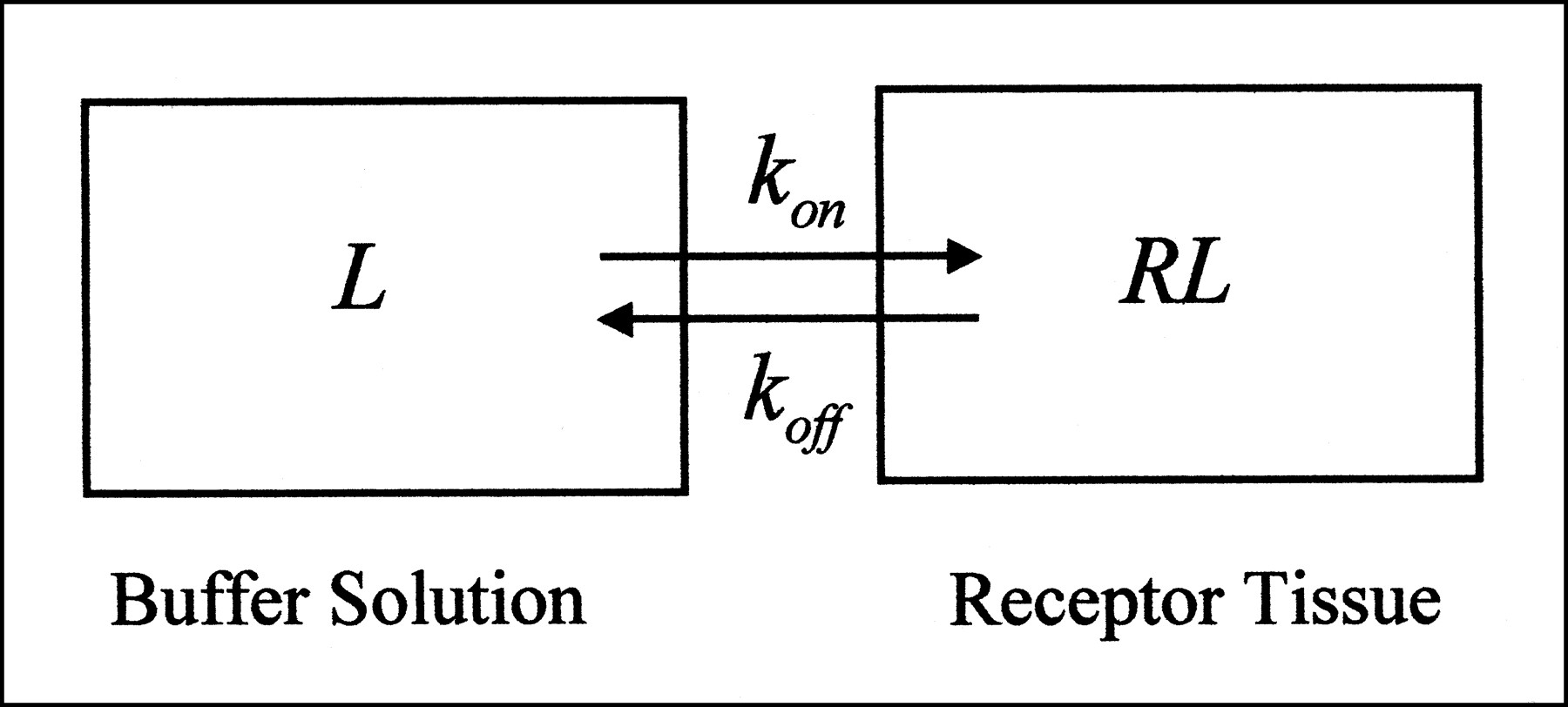
All of the modeling approaches in both radioligand binding assays and PET and SPECT studies assume a compartmental system. In radioligand binding assays, tissue homogenates are incubated in buffer solution with the radioligand (4). Hence, this type of experiment can be viewed as having two compartments (or is sometimes referred to as having one tissue compartment). One compartment reflects the buffer solution in the test tube, and the other reflects the receptor-rich tissue adjacent to the buffer (Fig. 1). Radioligands put into the test tube start in the buffer compartment and then can go directly into the tissue compartment by binding to receptors. This simplest model, describing the interaction of a receptor, R, with a radioligand, L, to form a complex, RL, is the bimolecular reaction described by Michaelis and Menton (5): $\text{[math]}$ Eq. 1 where [L] is the concentration of radioligand in buffer solution; [R] is the unbound receptor concentration; [RL] is the concentration of bound ligand to the receptor; and k_on and k_off are the association and dissociation kinetic rate constants, respectively. Reversibly binding radioligands reach equilibrium concentrations in buffer solution and tissue over time when no net transfer of radioligands occurs between the two compartments. After radioactivity-decay correction, all [L], [R], and [RL] remain constant because no other radioligands are lost from the system. According to the laws of mass reaction at equilibrium, $\text{[math]}$ Eq. 2 Because the equilibrium dissociation constant, K_d, is defined as k_off/k_on and the total number of receptors, B_max, is [R] + [RL], substitution for k_off/k_on and [R] in Equation 2 and rearrangement yields: $\text{[math]}$ Eq. 3 In a typical “saturation” radioligand binding assay experiment, increasing amounts of a radioligand are added to a fixed concentration of receptors, and [RL] is measured as a function of [L]. Nonlinear regression analysis can be used to fit Equation 3 to the data to estimate both B_max and K_d (4). Although it is also feasible to quantify both B_max and K_d separately by applying the same principle to in vivo PET and SPECT experiments (the exception is that a high concentration of “cold” ligands as opposed to radioligands is administered in additional experiments) (6), this approach not only would be impractical for routine use but also would be inappropriate for human studies because of the potentially undesirable pharmacologic effects.

FIGURE 1.

In vitro system consists of two compartments. Terms are defined in Appendix.

If an extremely small radioligand concentration is given, as is done with PET and SPECT studies, then [RL] is very small and, more important, [R] is approximately B_max (strictly speaking, [R] is referred to as B^′_max to distinguish it from B_max, which is [R] + [RL].) In this situation, Equation 2 can be rearranged to yield: $\text{[math]}$ Eq. 4 BP is defined as B_max/K_d and is equal to the ratio of bound radioligand concentration to free radioligand concentration at equilibrium. BP is proportional to B_max if K_d can be regarded as a constant.

PET and SPECT Studies

PET and SPECT studies differ from radioligand binding assays in two ways. First, brain regions containing receptors have at least three compartments (or are sometimes referred to as having two tissue compartments) (Fig. 2). Radioligands are given intravenously, go to the heart, and are then delivered in arterial blood. The first compartment is the arterial blood. From arterial blood, the radioligand passes through the blood–brain barrier into the second compartment, known as the free compartment. Anatomically, the free compartment probably consists of several regions, including interstitial fluid and intracellular cytoplasm. Even so, the free compartment is approximated as a single compartment. The third compartment is the region of specific binding that contains high-affinity receptors. Brain regions that do not have high-affinity receptors for the radioligand are referred to as reference regions and do not have the third compartment. There is also a nonspecific-binding compartment that exchanges with the free compartment. In practice, for most radioligands, the nonspecific-binding compartment is in rapid equilibrium with the free compartment and the two compartments are treated as a single compartment (often referred to as the nondisplaceable compartment).

FIGURE 2.

Two- and three-compartment configurations used to model in vivo radioligand kinetics. Terms are defined in Appendix.

Second, unlike the in vitro system, the in vivo system has an open first compartment, in that the radioligand in this compartment clears over time. Furthermore, delivery of the radioligand through this compartment to the second and hence to the third receptor compartment depends on regional cerebral blood flow. These two major differences between in vivo and in vitro studies make the former more complicated than the latter. However, the in vitro principle can be extended into the in vivo system.

Assumptions

In tracer kinetic modeling, certain fundamental or physiologically reasonable assumptions are usually made to minimize the number of kinetic parameters and yield reliable estimates of BP. Ultimately, the validity of such assumptions needs to be evaluated for any particular model. This topic is beyond the scope of this paper.

Usually, the following six assumptions are made for the compartment system:

Radioligand in the system comes from a single source, arterial plasma.
The radioligand can pass back and forth freely from arterial plasma to the free compartment.
First-order kinetics can describe the exchange of radioligand between compartments.
Nonspecifically bound radioactivity in the second compartment (C₂) equilibrates rapidly with free tissue radioactivity.
Unmetabolized parent radioligand in plasma equilibrates rapidly with plasma protein so that the free fraction (f₁) is constant over time (f₁ is defined below and in the Appendix).
The nondisplaceable distribution volume of C₂ (V^′₂) in the receptor-containing tissue is identical to the corresponding distribution volume (V₂) in the receptor-free tissue (V₂ and V^′₂ are defined below and in the Appendix).

Assumption 4 permits merging the free and nonspecific binding compartments into a single compartment. If the nonspecific compartment is considered separate, the compartment model can become much more difficult to solve reliably.

Tracer Kinetics

Thus, the in vivo system consists of the plasma compartment (C₁), the intracerebral nondisplaceable compartment (C₂), and the specifically bound receptor compartment (C₃) for receptor containing tissue; and C₁ and C^′₂ for the reference tissue (Fig. 2). This system can be described by the following set of differential equations (7): $\text{[math]}$ Eq. 5 $\text{[math]}$ Eq. 6 and $\text{[math]}$ Eq. 7 where K₁ and K^′₁ are delivery rate constants; k₂, k^′₂, k₃, and k₄ are the first-order kinetic rate constants; and C_P(t) is the total plasma concentration of radioligand. f₁ is the fraction of free (unbound to plasma proteins) unmetabolized parent radioligand activity in plasma, so that f₁C_P(t) represents the exchangeable portion of C₁. An alternative definition of f₁ found in many references is f₂ (defined in the Appendix).

BP

After a bolus injection, radioligand binding does not typically reach equilibrium. However, information acquired from scanning is used to derive the binding parameters that are found at equilibrium. At equilibrium, the left sides of Equations 5, 6, and 7 are all zero because no net transfer of radioligand occurs between the compartments. Hence, from Equation 5: $\text{[math]}$ Eq. 8 Substitution for C₂ from Equation 8 into Equation 6 at equilibrium and rearrangement yields: $\text{[math]}$ Eq. 9 Finally, from Equation 7: $\text{[math]}$ Eq. 10

The quantity of radioligand distributed in a compartment at equilibrium is referred to as the distribution volume, which is expressed as the equivalent volume of the plasma radioligand concentration at equilibrium. Thus, V₃ = C₃/f₁C_P = K₁k₃/k₂k₄, V₂ = C₂/f₁C_P = K₁/k₂, and V^′₂ = C^′₂/f₁C_P = K^′₁/k^′₂. The closest PET and SPECT equivalent for [RL]/[L] is C₃/f₁C_P, which is the BP (B_max/K_d) and is also V₃. Here, [L] in vitro is assumed to correspond to radioligand activity in plasma water. This definition of the BP proposed by Laruelle et al. (6,8) differs from the one originally proposed by Mintun et al. (7), in which BP was defined as B_max/K_d = k₃/k₄. The advantage of this definition is that PET- and SPECT-measured B_max and K_d values can be directly compared with those measured during in vitro radioligand binding assays.

Comparison of Equations 1, 2, 5, and 6 leads to the relationships between in vivo and in vitro systems, namely, k₃ ≠ k_on, but k₃ = (1/V₂)k_onB_max and k₄ = k_off (6,8). Quantification of BP = B_max/K_d = C₃/f₁C_P described so far requires blood data. Using the noninvasive quantification models described below, the best estimates of the receptor density are the ratio of V₃ to V₂, which is referred to as R_V, R_T (tissue ratio at equilibrium), V^′^′₃, or the “binding potential” (abbreviated here as BP* to distinguish it from BP = B_max/K_d). This binding potential, BP*, is related to BP and the kinetic parameters, k₃ and k₄, as follows: $\text{[math]}$ Eq. 11 For BP* to reflect the receptor density B_max, therefore, in addition to K_d, V₂ must be constant between individuals or disease conditions.

PET AND SPECT QUANTIFICATION MODELS

The differential equations, Equations 5, 6, and 7, are solved in several different ways so that they can be applied to PET and SPECT data. These solutions are referred to as quantification models or methods. Depending on the model, certain additional assumptions to those described above may be made to simplify the model. Some radioligands will meet certain assumptions better than others. Hence, the solutions from models in which the radioligand better meets the assumptions will have a better fit and be more reliable.

These models can be classified into two major categories depending on the ways in which radioligands are administered, namely, bolus or bolus plus constant infusion. The latter experimental paradigm attempts to achieve a sustained equilibrium by infusing radioligand at the same rate as that at which it is cleared from the first compartment (9–11). This paradigm actually simplifies receptor quantification because there is no need after all to solve the differential equations and the BP can be estimated directly from Equation 9. However, this approach is less widespread than the bolus-only paradigm because the infusion rate needed is influenced by radioligand delivery and clearance, which may vary between subjects. Furthermore, several hours of constant infusion are usually needed to achieve a sustained equilibrium.

This review therefore focuses on the models using the bolus injection paradigm. These models can be classified on the basis of whether arterial (more invasive) or reference (less invasive) data are needed. Some models use linear regression analysis as in graphic plots, whereas others use nonlinear regression analysis. Software packages are now available to apply these models to scanning data, even on a voxel-by-voxel basis (12,13).

GRAPHIC MODELS

The graphic models generally allow quick estimation of the BP by graphically fitting a straight line to experimental data or using linear regression analysis.

Logan Invasive Plot

In PET and SPECT, regions of brain tissue are sampled by drawing an ROI. The radioactivities in an ROI at time t within reference (C_RF(t)) and receptor-rich (C_RC(t)) brain tissues can be expressed as C_RF(t) = C^′₂(t) + C_P(t)V₁ and C_RC(t) = C₂(t) + C₃(t) + C_P(t)V₁, respectively, where V₁ is the vascular volume within the ROI. V₁ is estimated at 5% and often has a negligible contribution after the initial part of the study because the typical plasma time–activity curve has an immediate high peak followed by very low concentrations (Fig. 4). For the two-compartment region, integration of both sides of Equation 7 and rearrangement yields: $\text{[math]}$ Eq. 12 Substitution for C^′₂(t) = C_RF(t) − C_P(t)V₁ and V^′₂ = K^′₁/k^′₂ and division of both sides of Equation 12 by C_RF(t) followed by rearrangement yields: $\text{[math]}$ Eq. 13 $\text{[math]}$ After the initial period, the plot of ∫₀^t C_RF(t)dt/C_RF(t) versus ∫₀^t C_P(t)dt/C_RF(t) is linear, with a slope a′ = V^′₂f₁ and an intercept b′ = 1/k₂, because V^′₂ >> V₁, and the contribution of V₁C_P(t)/C_RF(t) is small.

Similarly, for the three-compartment region the following solution can be obtained from Equations 5 and 6. Logan et al. and others (14–17) have shown that the last term in this Equation 14 becomes constant (b) after a certain time, t*, when a steady state condition exists such that C₂(t)/C_P(t) and C₃(t)/C_P(t) are constant: $\text{[math]}$ Eq. 14 Thus, a plot of ∫₀^t C_RC(t)dt/C_RC(t) versus (∫₀^t C_P(t)dt)/C_RC(t)dt has slope a = f₁V₂ + f₁V₃ + V₁ and intercept b. If we assume V^′₂ = V₂ (assumption 6) and neglect V₁, the binding potentials BP and BP* are given by BP = f₁(a − a′) and BP* = a/a′ − 1, respectively.

Noninvasive Plots

Logan Noninvasive Plot.

Logan et al. (18) showed two noninvasive models (Eqs. 15 and 16) to estimate the distribution volume ratio, DVR, which equals (V₂ + V₃)/V₂ (or BP* + 1). Because C_RC(t) = C₂(t) + C₃(t) + C_P(t)V₁ and C_RF(t) = C^′₂(t) + C_P(t)V₁, by substituting C_RF(t) for (C₂(t) + C_P(t)V₁), one can write Equation 14 as: $\text{[math]}$ Eq. 15 $\text{[math]}$ where δ(t) denotes the vascular effect within the ROI. δ(t) becomes relatively constant over time. Eventually, the plot of ∫₀^t C_RC(t)dt/C_RC(t) versus (∫₀^t C_RF(t)dt−C_RF(t)/k^′₂)C_RC(t) becomes linear, with slope DVR = BP* + 1 = a/a′ =(V₂ + V₃)/V₂ (V₁ is neglected here, and V^′₂ = V₂, as shown above). Use of Equation 15 requires that k^′₂ be taken from an independent population sample and assumed to be representative for the individual subject scanned. Estimation of k^′₂ requires the invasive model (k^′₂ = −1/b′ in Eq. 13).

If C_RF(t)/C_RC(t) becomes constant, then k^′₂ is not needed because Equation 15 can be simplified to (18): $\text{[math]}$ Eq. 16 The plot of ∫₀^t C_RC(t)dt/C_RC(t) versus ∫₀^t C_RF(t)dt/C_RC(t) then becomes linear, and the slope gives DVR. Although the predetermined value of k^′₂ is not required, C_RF(t)/C_RC(t) must be shown to become constant during the scanning period. The validity of these additional assumptions for the Logan noninvasive plots depends on the radioligand.

Ichise Noninvasive Plot.

Solving for the plasma term, ∫₀^t C_P(t)dt, in Equation 13 and inserting it into Equation 14 (19,20) gives: $\text{[math]}$ Eq. 17 Equation 17 is a multilinear equation beyond time t*. Thus, BP* = a/a − 1 can be estimated by multilinear regression analysis (19,20). t* is determined by setting the allowable variance in the regression. With regression analysis, the value of each time point has a residual value indicating the deviation of the observed value from the expected value. Early time values are excluded on the basis of the size of the residuals (21). Unlike Logan plots, this model does not require the value of k^′₂ or the assumption that C_RF(t)/C_RC(t) becomes constant during the scanning period.

NONGRAPHIC MODELS

In contrast to the graphic models, some of the nongraphic models require technically demanding nonlinear regression analysis to estimate the BP and other kinetic parameters (22).

Kinetic Analysis Invasive Model

Here, the linear first-order differential equations (Eqs. 5, 6, and 7) are solved directly. Frost et al. (23) described the solution as follows: $\text{[math]}$ Eq. 18 C_ROI(t) = C_RF(t) for the two-compartment region, and C_ROI(t) = C_RC(t) for the three-compartment region. “m” is the number of tissue compartments. The number of tissue compartments is the total number of compartments minus one. ⊗ represents a convolution (Appendix).

For the two-compartment region, L₁ = K^′₁ and R₁ = k^′₂. For the three-compartment region, $\text{[math]}$ and $\text{[math]}$ BP, BP*, and individual kinetic parameters are estimated using nonlinear regression analysis to fit Equation 18 to the time–activity data. As in the graphic models, V^′₂ = K^′₁/k^′₂ is first estimated in the reference region, and this value is substituted for K₁/k₂ in Equation 10 before nonlinear fitting. This substitution reduces the number of parameters for the three-compartment region and usually makes the parameter estimation more stable. In contrast to the linear regression analysis used in the graphic models, however, if the selection of the initial parameter values is inappropriate, the nonlinear minimization process may fail to converge or may become trapped in “local” minima rather than finding the “global” minima, yielding false parameter values (24). Cunningham and Lammertsma (25) provided further detail on this invasive model.

Noninvasive Models

Lammertsma Reference Tissue Model.

Solving for the plasma term, C_P(t), in Equation 7; inserting the plasma term into Equations 5 and 6; and expressing the parameters in terms of R_I, k₂, k₃, and BP* yield a set of new differential equations that can be solved directly as in the kinetic analysis model, in which R_I = K₁/K^′₁ and k₂/R_I has been substituted for k^′₂ with the assumption that K′1/k^′₂ = K^′₁/k^′₂ (26). However, because nonlinear fitting of this solution can be unstable, another assumption is made to reduce the number of parameters to R_I, k₂, and BP*. That assumption is that the radioligand kinetics in the region of specific binding can be approximated to a single tissue compartment so that the free and specific binding compartments are considered one compartment. For this approximation to occur, k₃ and k₄ should reflect rapid exchange in comparison with K₁ and k₂.

The final solution Lammertsma and Hume (26) derived is: $\text{[math]}$ Eq. 19 $\text{[math]}$ As in the kinetic analysis model, the Lammertsma model requires technically demanding nonlinear fitting of experimental data.

Basis Function Model.

Modeling each voxel as a separate ROI within an image is computationally labor intensive. For decay-corrected data, Gunn et al. (13) proposed to reduce the simplified reference tissue model (26) (Eq. 19) as: $\text{[math]}$ Eq. 20 where θ₁ = R_I, θ₂ = (k₂ − R_Ik₂/(1 + BP*)), θ₃ = k₂t/(1 + BP*), and the basis function is defined as B_i(t) = C_ref(t) ⊗ e^−0_3i(t). B_i(t) can be determined by choosing a range of plausible values for θ₃ based on solutions from ROI data. Gunn et al. used 100 values for B_i and a logarithmic range of values for θ₃. With boundary estimates for θ₁ and θ₂, Equation 20 can be fitted more quickly with a linear least squares approach. The assumptions required for this model are those required for the simplified reference region model. Additional assumptions are that the B_i chosen is appropriate for solving the equation, that the number of discrete values for B_i is adequate, and that the boundaries set for estimated maximum and minimum values for θ₁, θ₂, and θ₃ based on ROI data reflect the boundaries for these parameters at the voxel level.

Peak Equilibrium Model.

The major additional assumption for this model is that C^′₂(t) in the reference region is the same as C₂(t) in the region of specific binding (this assumption is not the same as V^′₂ = V₂). Given that radioligand goes from the free compartment to the specific compartment in the region of specific binding, this assumption is unlikely to be perfectly true. However, for some radioligands, the assumption is sufficiently valid to derive the BP (27). Because C_RC(t) = C₂(t) + C₃(t) + C_P(t)V₁ and C_RF(t) = C^′₂(t) + C_P(t)V₁, if C₂(t) = C^′₂(t) then C_RC(t) − C_RF(t) = C₃(t), and C₃(t) may be plotted and a curve fitted to these data. At the peak of the fitted curve, dC₃(t)/dt = 0, hence C₃(t)/C_RF(t) = BP* = k₃/k₄. A variation of this model applies to the case of ¹²³I-2β-carbomethoxy-3β-(4-iodophenyl)tropane ([¹²³I]β-CIT), a SPECT dopamine transporter tracer in which the radioligand kinetics are so slow that a protracted peak equilibrium is reached 24 h after injection and only one scan during this prolonged equilibrium is needed to estimate BP* (28).

Transient Equilibrium (Ratio) Model.

For certain radioligands, the tissue ratio C_RC(t)/C_RF(t) can become constant over time after a bolus injection of radioligand. This state is called a pseudo or transient equilibrium. As in the peak equilibrium model, if we assume that C^′₂(t) = C₂(t) during this transient equilibrium, then BP* = C_RC(t)/C_RF(t) − 1. However, C₂(t) is often less than C^′₂(t), and Carson et al. (29) have shown that this model may overestimates BP*.

MODEL COMPARISONS

The advantages of invasive models are as follows:

Invasive models allow estimation of BP = B_max/K_d rather than BP* = BP/V₂, although the latter can also be estimated. When V₂ has a large intersubject variability, an invasive model is essential for between-subject comparisons.
Under conditions in which no reference region is available, a measure related to B_max/K_d may still be detectable if V₂ has a low variability between subjects. For example, V_T = V₃ + V₂ can be estimated and, if V₂ is constant, should reflect the receptor density.
Generally, invasive models have fewer assumptions than do noninvasive models.

The disadvantages of invasive models are as follows:

Arterial sampling is invasive, is associated with discomfort, and is technically demanding.
The arterial sample comes from a coincidence detector that is different from the PET scanner. Although the detector can be calibrated, the variance of the measurement may differ.
Accurate measurement of metabolites in plasma is required to determine the concentration of parent radioligand in plasma and requires additional staffing during scanning.
Accurate measurement of the free-fraction f₁ is also required.
The arterial sample measurement often has greater variance (in part as a result of disadvantages 2, 3, and 4). Although arterial sampling models may be more accurate, they may often be less reproducible.

Table 1 (30) compares the assumptions required for each noninvasive model. If the kinetics of the radioligand allow the assumptions for a valid model, the model is suitable for that radioligand.

View this table:

TABLE 1

Assumption Requirement for Noninvasive Models

The following illustrates the choice of noninvasive models. A dataset of SPECT using [¹²³I]iodobenzofuran (IBF, a dopamine D₂ receptor tracer) was acquired for a healthy person and a person with possible multiple-system atrophy. Sample IBF SPECT images and time–activity data are shown in Figures 3 and 4, respectively (30). How does one choose an appropriate model to analyze the data? The frontal cortex is known to have the properties of a reference region for IBF (19). Also known is that V₂ does not vary for this radioligand between subjects (31). Given this information, several noninvasive models are potentially suitable. Clearance of IBF is known to have a high intersubject variability, and t* is known to be reasonably early (19). The use of a single tissue compartment is unclear for this radioligand. In view of the assumptions in Table 1, the models that appear potentially suitable include the Logan noninvasive and the Ichise noninvasive. Table 2 (30) shows the BP* values calculated from the IBF SPECT dataset described in Figure 4. Some models show discrepant results that may be attributed to inadequately met assumptions.

FIGURE 3.

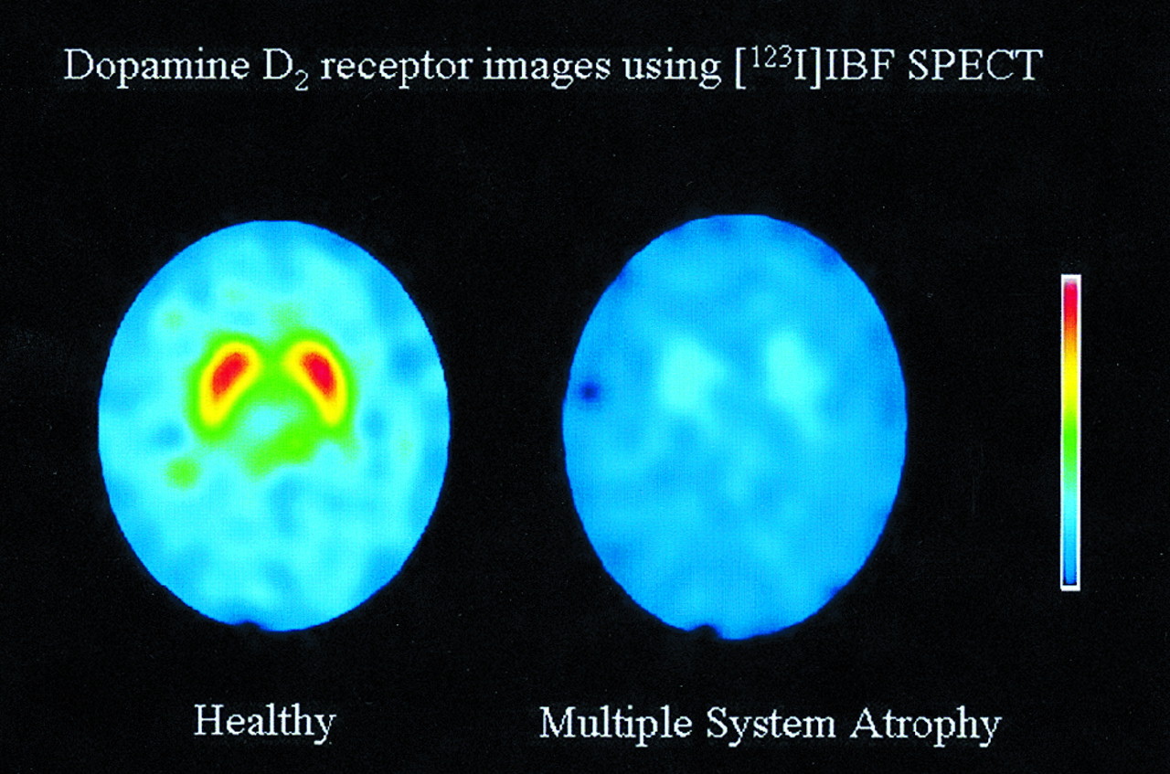
Selected [¹²³I]IBF dopamine D₂ receptor images of healthy individual (left) and patient with multiple-system atrophy (right). Paired central activity reflects striatal dopamine D₂ binding, which is markedly reduced in patient. (Reprinted with permission of (30).)

FIGURE 4.

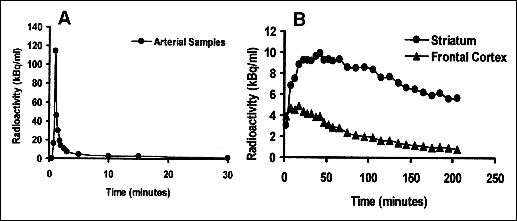
Plasma (A) and brain ROI (B) time–activity curves from [¹²³I]IBF SPECT study of healthy individual. (Reprinted with permission of (30).)

View this table:

TABLE 2

Binding Potential Values for [¹²³I]IBF SPECT from Single Dataset

CONCLUSION

Tracer kinetic modeling in PET and SPECT allows the derivation of equilibrium parameters that describe radioligand-receptor kinetics such as the BP and the V₃/V₂ from time–activity data. These parameters are related to B_max and K_d, which are traditionally found by in vitro radioligand binding assays. Such data may be used to assess the neuropathology of diseases that change B_max or K_d. Recent developments in modeling reversible ligands have generated several noninvasive approaches that can readily be applied to provide quantitative data, provided that the radioligand adequately meets the assumptions inherent in the model used.

APPENDIX

Definitions of Terms

[L]:: Concentration of unbound radioligand in buffer solution (Bq/mL). [L] corresponds to f₁C_P(t).
[RL]:: Concentration of bound radioligand (Bq/mL). [RL] corresponds to C₃(t).
[R], B^′_max:: Concentration of unbound receptors (mol/g). [R] = B^′_max, which is nearly equal to B_max when the radioligand is used at tracer doses.
B_max:: Concentration of receptors (mol/g). B_max = [R] + [RL].
k_on, k_off:: Association and dissociation rate constants, respectively, for the bimolecular reaction.
K_d:: Equilibrium dissociation constant for the radioligand–binding site complex. K_d = k_off/k_on measured in aqueous solution, either the solvent in the case of in vitro radioligand binding assays or plasma water in the case of PET and SPECT.
C_P(t):: Plasma activity of unmetabolized parent radioligand (Bq/mL).
f₁:: Free fraction of plasma unmetabolized parent radioligand.
f₂:: fraction of free compartment from which the radioligand can exchange with the specifically bound compartment.
C^′₂(t), C₂(t):: Tissue radioligand activity in the nondisplaceable compartment (Bq/mL) for reference and receptor-containing tissues, respectively.
C₃(t):: Tissue radioligand activity bound to receptors (Bq/mL).
C_RF(t):: Tissue radioligand activity in the receptor-devoid reference region of interest, including plasma activity (Bq/mL). C_RF(t) = C^′₂(t) + C_P(t)V₁.
C_RC(t):: Tissue radioligand activity in the receptor-containing region of interest, including plasma activity (Bq/mL). C_RC(t) = C₂(t) + C₃(t) + C_P(t)V₁.
K₁, K^′₁:: Transfer constants from plasma to tissue for receptor-containing and reference tissues, respectively (mL/g/min), which are the product of regional blood flow (F) and unidirectional extraction fraction (E).
k₂, k^′₂:: Transfer constants from tissue to plasma for receptor-containing and reference tissues, respectively (per minute).
k₃, k₄:: Transfer constants between second and third compartments (per minute). k₃ = (1/V₂)k_onB_max and k₄ = k_off.
V₁:: Plasma volume (milliliters) in 1 g of tissue.
V^′₂, V₂:: Nondisplaceable distribution volumes, which are assumed to be the same for reference (V^′₂) and receptor-containing (V₂) tissues, defined as V^′₂ = V₂ = K₁/k₂ = K^′₁/k^′₂ (mL/g). K₁/k₂ is also referred to as the partition coefficient (λ)
V₃:: Distribution volume of C₃ or binding potential defined as V₃ = B^′_max/K_d = B_max/K_d = K₁k₃/k₂k₄ (mL/g).
V_T:: Total-volume distribution volume in a receptor-containing brain region, defined as V_T = V₂f₁ + V₃f₁ + V₁.
BP:: The binding potential defined as V₃ = K₁k₃/k₂k₄ = B_max/K_d.
BP*:: Another definition of binding potential, defined as BP* = V₃/V₂ = BP/V₂ = B_max/V₂K_d = k₃/k₄.
R_V, R_T, V^′^′₃, DVr:: Distribution volume ratio, R_V; equilibrium tissue ratio, R_T; and V^′^′₃ are the same as BP*. Another distribution volume ratio, DVr, is equal to (V₂ + V₃)/V₂ = BP* + 1.
R_I:: R_I = K₁/K^′₁.
⊗:: Convolution, a mathematic expression that can be defined using functions f and g as follows: f ⊗ g= ∫₀^t f(t−τ)g(τ)dτ.

Acknowledgments

This study was supported by the Ministry of Education Science and Culture of Japan (Foreign Visiting Scientist Program), the Medical Research Council of Canada, the National Alliance for Research in Schizophrenia and Depression, and the Japan Society for the Promotion of Sciences (JSPS-RFTF97L00203).

Footnotes

Received Oct. 19, 2000; revision accepted Jan. 16, 2001.
For correspondence or reprints contact: Masanori Ichise, MD, Room B3-10 MIB-NIMH, Bldg. One, 1 Center Dr. MSC 0135, Bethesda, MD 20892-0135.
*NOTE: FOR CE CREDIT, YOU CAN ACCESS THIS ACTIVITY THROUGH THE SNM WEB SITE (http://www.snm.org/education/ce_online.html) UNTIL MAY 2002.

REFERENCES

↵
Volkow ND, Fowler JS, Gatley SJ, et al. PET evaluation of the dopamine system of the human brain. J Nucl Med. 1996;37:1242–1256.
Marek KL, Seibyl JP, Zoghbi SS, et al. [¹²³I] beta-CIT/SPECT imaging demonstrates bilateral loss of dopamine transporters in hemi-Parkinson’s disease. Neurology. 1996;46:231–237.
↵
Ichise M, Kim YJ, Ballinger JR, et al. SPECT imaging of pre- and postsynaptic dopaminergic alterations in L-dopa-untreated PD. Neurology. 1999;52:1206–1214.
↵
McGonigle P, Molinoff PB. Receptors and signal transduction: classification and quantitation. In: Siegel GJ, Agranoff BW, Albers RW, Molinoff PB, eds. Basic Neurochemistry. New York, NY: Raven Press; 1994:209–230.
↵
Michaelis L, Menten ML. Die Kinetik der Invertinwirkung. Biochem Z. 1913;49:1333.
↵
Laruelle M, al-Tikriti MS, Zea-Ponce Y, et al. In vivo quantification of dopamine D2 receptor parameters in nonhuman primates with [¹²³I]iodobenzofuran and single photon emission computerized tomography. Eur J Pharmacol. 1994;263:39–51.
↵
Mintun MA, Raichle ME, Kilbourn MR, Wooten GF, Welch MJ. A quantitative model for the in vivo assessment of drug binding sites with positron emission tomography. Ann Neurol. 1984;15:217–227.
↵
Laruelle M, van Dyck C, Abi-Dargham A, et al. Compartmental modeling of iodine-123-iodobenzofuran binding to dopamine D2 receptors in healthy subjects. J Nucl Med. 1994;35:743–754.
↵
Laruelle M, Baldwin RM, Rattner Z, et al. SPECT quantification of [¹²³I]iomazenil binding to benzodiazepine receptors in nonhuman primates. I. Kinetic modeling of single bolus experiments. J Cereb Blood Flow Metab. 1994;14:439–452.
Abi-Dargham A, Laruelle M, Seibyl J, et al. SPECT measurement of benzodiazepine receptors in human brain with iodine-123-iomazenil: kinetic and equilibrium paradigms. J Nucl Med. 1994;35:228–238.
↵
Carson RE, Channing MA, Blasberg RG, et al. Comparison of bolus and infusion methods for receptor quantitation: application to [¹⁸F] cyclofoxy and positron emission tomography. J Cereb Blood Flow Metab. 1993;13:24–42.
↵
Berger C, Buck A. Requirements and implementation of a flexible kinetic modeling tool. J Nucl Med. 1997;38:1818–1823.
↵
Gunn RN, Lammertsma AA, Hume SP, Cunningham VJ. Parametric imaging of ligand-receptor binding in PET using a simplified reference region model. Neuroimage. 1997;6:279–287.
↵
Patlak CS, Blasberg RG, Fenstermacher JD. Graphical evaluation of blood-to-brain transfer constants from multiple-time uptake data. J Cereb Blood Flow Metab. 1983;3:1–7.
Gjedde A. High- and low-affinity transport of D-glucose from blood to brain. J Neurochem. 1981;36:1463–1471.
Logan J, Fowler JS, Volkow ND, et al. Graphical analysis of reversible radioligand binding from time-activity measurements applied to [N-¹¹C-methyl]-(-)-cocaine PET studies in human subjects. J Cereb Blood Flow Metab. 1990;10:740–747.
↵
Patlak CS, Blasberg RG. Graphical evaluation of blood-to-brain transfer constants from multiple-time uptake data: generalizations. J Cereb Blood Flow Metab. 1985;5:584–590.
↵
Logan J, Fowler JS, Volkow ND, Wang GJ, Ding YS, Alexoff DL. Distribution volume ratios without blood sampling from graphical analysis of PET data. J Cereb Blood Flow Metab. 1996;16:834–840.
↵
Ichise M, Ballinger JR, Golan H, et al. Noninvasive quantification of dopamine D2 receptors with iodine-123-IBF SPECT. J Nucl Med. 1996;37:513–520.
↵
Ichise M, Ballinger JR. From graphical analysis to multilinear regression analysis of reversible radioligand binding [letter]. J Cereb Blood Flow Metab. 1996;16:750–752.
↵
Ichise M, Ballinger JR, Vines D, Tsai S, Kung HF. Simplified quantification and reproducibility studies of dopamine D2-receptor binding with iodine-123-IBF SPECT in healthy subjects. J Nucl Med. 1997;38:31–37.
↵
Carson RE. Parameter estimation in positron emission tomography. In: Phelps ME Mazziota JC, Schelbert HR, eds. Positron Emission Tomography: Principles and Applications for the Brain and the Heart. New York, NY: Raven Press; 1986:347–390.
↵
Frost JJ, Douglass KH, Mayberg HS, et al. Multicompartmental analysis of [¹¹C]-carfentanil binding to opiate receptors in humans measured by positron emission tomography. J Cereb Blood Flow Metab. 1989;9:398–409.
↵
Motulsky HJ, Ransnas LA. Fitting curves to data using nonlinear regression: a practical and nonmathematical review. FASEB J. 1987;1:365–374.
↵
Cunningham V, Lammertsma A. Radioligand studies in brain: kinetic analysis of PET data. Med Chem Res. 1994;5:79–96.
↵
Lammertsma AA, Hume SP. Simplified reference tissue model for PET receptor studies. Neuroimage. 1996;4:153–158.
↵
Farde L, Eriksson L, Blomquist G, Halldin C. Kinetic analysis of central [¹¹C]raclopride binding to D2-dopamine receptors studied by PET: a comparison to the equilibrium analysis. J Cereb Blood Flow Metab. 1989;9:696–708.
↵
Laruelle M, Wallace E, Seibyl JP, et al. Graphical, kinetic, and equilibrium analyses of in vivo [¹²³I]β-CIT binding to dopamine transporters in healthy human subjects. J Cereb Blood Flow Metab. 1994;14:982–994.
↵
Carson RE, Channing MA, Blasberg RG, et al. Comparison of bolus and infusion methods for receptor quantitation: application to [¹⁸F]cyclofoxy and positron emission tomography. J Cereb Blood Flow Metab. 1993;13:24–42.
↵
Meyer JH, Ichise M. Modeling of receptor ligand data in PET and SPECT imaging: a review of major approaches. J Neuroimaging. 2001;11:30–39.
↵
Ichise M, Fujita M, Seibyl JP, et al. Graphical analysis and simplified quantification of striatal and extrastriatal dopamine D₂ receptor binding with [¹²³I]epidepride SPECT. J Nucl Med. 1999;40:1902–1912.

[1] ↵
Volkow ND, Fowler JS, Gatley SJ, et al. PET evaluation of the dopamine system of the human brain. J Nucl Med. 1996;37:1242–1256.

[2] Marek KL, Seibyl JP, Zoghbi SS, et al. [¹²³I] beta-CIT/SPECT imaging demonstrates bilateral loss of dopamine transporters in hemi-Parkinson’s disease. Neurology. 1996;46:231–237.

[3] ↵
Ichise M, Kim YJ, Ballinger JR, et al. SPECT imaging of pre- and postsynaptic dopaminergic alterations in L-dopa-untreated PD. Neurology. 1999;52:1206–1214.

[4] ↵
McGonigle P, Molinoff PB. Receptors and signal transduction: classification and quantitation. In: Siegel GJ, Agranoff BW, Albers RW, Molinoff PB, eds. Basic Neurochemistry. New York, NY: Raven Press; 1994:209–230.

[5] ↵
Michaelis L, Menten ML. Die Kinetik der Invertinwirkung. Biochem Z. 1913;49:1333.

[6] ↵
Laruelle M, al-Tikriti MS, Zea-Ponce Y, et al. In vivo quantification of dopamine D2 receptor parameters in nonhuman primates with [¹²³I]iodobenzofuran and single photon emission computerized tomography. Eur J Pharmacol. 1994;263:39–51.

[7] ↵
Mintun MA, Raichle ME, Kilbourn MR, Wooten GF, Welch MJ. A quantitative model for the in vivo assessment of drug binding sites with positron emission tomography. Ann Neurol. 1984;15:217–227.

[8] ↵
Laruelle M, van Dyck C, Abi-Dargham A, et al. Compartmental modeling of iodine-123-iodobenzofuran binding to dopamine D2 receptors in healthy subjects. J Nucl Med. 1994;35:743–754.

[9] ↵
Laruelle M, Baldwin RM, Rattner Z, et al. SPECT quantification of [¹²³I]iomazenil binding to benzodiazepine receptors in nonhuman primates. I. Kinetic modeling of single bolus experiments. J Cereb Blood Flow Metab. 1994;14:439–452.

[10] Abi-Dargham A, Laruelle M, Seibyl J, et al. SPECT measurement of benzodiazepine receptors in human brain with iodine-123-iomazenil: kinetic and equilibrium paradigms. J Nucl Med. 1994;35:228–238.

[11] ↵
Carson RE, Channing MA, Blasberg RG, et al. Comparison of bolus and infusion methods for receptor quantitation: application to [¹⁸F] cyclofoxy and positron emission tomography. J Cereb Blood Flow Metab. 1993;13:24–42.

[12] ↵
Berger C, Buck A. Requirements and implementation of a flexible kinetic modeling tool. J Nucl Med. 1997;38:1818–1823.

[13] ↵
Gunn RN, Lammertsma AA, Hume SP, Cunningham VJ. Parametric imaging of ligand-receptor binding in PET using a simplified reference region model. Neuroimage. 1997;6:279–287.

[14] ↵
Patlak CS, Blasberg RG, Fenstermacher JD. Graphical evaluation of blood-to-brain transfer constants from multiple-time uptake data. J Cereb Blood Flow Metab. 1983;3:1–7.

[15] Gjedde A. High- and low-affinity transport of D-glucose from blood to brain. J Neurochem. 1981;36:1463–1471.

[16] Logan J, Fowler JS, Volkow ND, et al. Graphical analysis of reversible radioligand binding from time-activity measurements applied to [N-¹¹C-methyl]-(-)-cocaine PET studies in human subjects. J Cereb Blood Flow Metab. 1990;10:740–747.

[17] ↵
Patlak CS, Blasberg RG. Graphical evaluation of blood-to-brain transfer constants from multiple-time uptake data: generalizations. J Cereb Blood Flow Metab. 1985;5:584–590.

[18] ↵
Logan J, Fowler JS, Volkow ND, Wang GJ, Ding YS, Alexoff DL. Distribution volume ratios without blood sampling from graphical analysis of PET data. J Cereb Blood Flow Metab. 1996;16:834–840.

[19] ↵
Ichise M, Ballinger JR, Golan H, et al. Noninvasive quantification of dopamine D2 receptors with iodine-123-IBF SPECT. J Nucl Med. 1996;37:513–520.

[20] ↵
Ichise M, Ballinger JR. From graphical analysis to multilinear regression analysis of reversible radioligand binding [letter]. J Cereb Blood Flow Metab. 1996;16:750–752.

[21] ↵
Ichise M, Ballinger JR, Vines D, Tsai S, Kung HF. Simplified quantification and reproducibility studies of dopamine D2-receptor binding with iodine-123-IBF SPECT in healthy subjects. J Nucl Med. 1997;38:31–37.

[22] ↵
Carson RE. Parameter estimation in positron emission tomography. In: Phelps ME Mazziota JC, Schelbert HR, eds. Positron Emission Tomography: Principles and Applications for the Brain and the Heart. New York, NY: Raven Press; 1986:347–390.

[23] ↵
Frost JJ, Douglass KH, Mayberg HS, et al. Multicompartmental analysis of [¹¹C]-carfentanil binding to opiate receptors in humans measured by positron emission tomography. J Cereb Blood Flow Metab. 1989;9:398–409.

[24] ↵
Motulsky HJ, Ransnas LA. Fitting curves to data using nonlinear regression: a practical and nonmathematical review. FASEB J. 1987;1:365–374.

[25] ↵
Cunningham V, Lammertsma A. Radioligand studies in brain: kinetic analysis of PET data. Med Chem Res. 1994;5:79–96.

[26] ↵
Lammertsma AA, Hume SP. Simplified reference tissue model for PET receptor studies. Neuroimage. 1996;4:153–158.

[27] ↵
Farde L, Eriksson L, Blomquist G, Halldin C. Kinetic analysis of central [¹¹C]raclopride binding to D2-dopamine receptors studied by PET: a comparison to the equilibrium analysis. J Cereb Blood Flow Metab. 1989;9:696–708.

[28] ↵
Laruelle M, Wallace E, Seibyl JP, et al. Graphical, kinetic, and equilibrium analyses of in vivo [¹²³I]β-CIT binding to dopamine transporters in healthy human subjects. J Cereb Blood Flow Metab. 1994;14:982–994.

[29] ↵
Carson RE, Channing MA, Blasberg RG, et al. Comparison of bolus and infusion methods for receptor quantitation: application to [¹⁸F]cyclofoxy and positron emission tomography. J Cereb Blood Flow Metab. 1993;13:24–42.

[30] ↵
Meyer JH, Ichise M. Modeling of receptor ligand data in PET and SPECT imaging: a review of major approaches. J Neuroimaging. 2001;11:30–39.

[31] ↵
Ichise M, Fujita M, Seibyl JP, et al. Graphical analysis and simplified quantification of striatal and extrastriatal dopamine D₂ receptor binding with [¹²³I]epidepride SPECT. J Nucl Med. 1999;40:1902–1912.

Main menu

User menu

Search

An Introduction to PET and SPECT Neuroreceptor Quantification Models*

Abstract