


Abstract
The aim of this work was to find an optimal setup for activity determination of 177Lu-based SPECT/CT imaging reconstructed with 2 commercially available methods (xSPECT Quant and Flash3D). For this purpose, 3-dimensional (3D)–printed phantoms of different geometries were manufactured, different partial-volume correction (PVC) methods were applied, and the accuracy of the activity determination was evaluated. Methods: A 2-compartment kidney phantom (70% cortical and 30% medullary compartment), a sphere, and an ellipsoid of equal volumes were 3D printed, filled with 177Lu, and scanned with a SPECT/CT system. Reconstructions were performed with xSPECT and Flash3D. Different PVC methods were applied to find an optimal quantification setup: method 1 was a geometry-specific recovery coefficient based on the 3D printing model, method 2 was a geometry-specific recovery coefficient based on the low-dose CT scan, method 3 was an enlarged volume of interest including spilled-out counts, method 4 was activity concentration in the peak milliliter applied to the entire CT-based volume, and method 5 was a fixed threshold of 42% of the maximum in a large volume containing the object of interest. Additionally, the influence of postreconstruction gaussian filtering was investigated. Results: Although the recovery coefficients of sphere and ellipsoid differed by only 0.7%, a difference of 31.7% was observed between the sphere and the renal cortex phantoms. Without postfiltering, the model-based recovery coefficients (methods 1 and 2) resulted in the best accuracies (xSPECT, 1.5%; Flash3D, 10.3%), followed by the enlarged volume (method 3) (xSPECT, 8.5%; Flash3D, 13.0%). The peak-milliliter method (method 4) showed large errors only for sphere and ellipsoid (xSPECT, 23.4%; Flash3D, 21.6%). Applying a 42% threshold (method 5) led to the largest quantification errors (xSPECT, 32.3%; Flash3D, 46.7%). After postfiltering, a general increase in the errors was observed. Conclusion: In this work, 3D printing was used as a prototyping technique for a geometry-specific investigation of SPECT/CT reconstruction parameters and PVC methods. The optimal setup for activity determination was found to be an unsmoothed SPECT/CT reconstruction in combination with a recovery coefficient based on the low-dose CT. The difference between spheric and renal recovery coefficients suggests that the typically applied volume-dependent but only sphere-based recovery coefficient lookup tables should be replaced by a more geometry-specific alternative.
- radionuclide therapy
- 2-compartment kidney phantom
- 3D printing
- partial volume correction
- quantitative SPECT/CT
- xSPECT Quant
Quantitative assessment of radioactivity distributions is critical for planning and monitoring of molecular radiotherapies (MRT) based on internal dosimetry. With numerous improvements of the reconstruction procedure (1–3), quantitative SPECT/CT has recently evolved into one of the most widely used imaging modalities for estimating organ activities or activity concentrations (4–7), in particular for MRT (8). Despite its great potential, however, SPECT/CT still has some disadvantages considerably complicating a volume-of-interest (VOI)–based activity determination. Most importantly, the poor spatial resolution (in the centimeter range) leads to a major impact of the so-called partial-volume effect—a resolution-induced displacement of counts. The partial-volume effect is a combination of spill-out of counts originating in an object of interest to regions adjacent to the object and spill-in of counts originating in the background or adjacent objects into the object’s volume. In the absence of background (i.e., no spill-in), the result is an underestimation of the activity in any object-based VOI. Many efforts have been made to compensate for partial-volume effects (9). Image enhancement techniques seek to recover the resolution directly from the emission data. Here, resolution modeling can be performed either during the image reconstruction (10–12) or as postprocessing (13,14). In contrast, image-domain correction techniques rely on anatomic information or predetermined experimental findings to correct for partial volume (15–17). As an example, it is a common practice in oncologic applications to account for partial-volume effects by applying volume-specific recovery coefficients that are experimentally predetermined using spheric phantom inserts (15,18,19). Despite these efforts, the estimation of whole-organ activities remains a challenge.
To ensure reliable dosimetry for targeted radiotherapy based on planar and SPECT/CT imaging, partial-volume errors can be assessed through quasirealistic anthropomorphic phantoms of a known activity (6,7,20). Because industrial manufacturing of such phantoms is expensive and profitable only for producing larger quantities, only few phantoms—typically spheres and cylinders—are commercially available.
To overcome this limitation, the potential of low-cost 3-dimension (3D) printing for the fabrication of fillable organ phantoms has been demonstrated recently (21,22). In our previous study (21), the kidney, as the critical organ in many radionuclide therapies using 90Y- or 177Lu-labeled compounds (23,24), was investigated. No relevant differences in partial-volume behavior were found between a set of single-compartment kidneys (25) and spheres of the same volumes. In addition, an investigation of different organ phantoms was performed by Robinson et al. (22), suggesting that spill-out effects become more relevant in organs, such as the pancreas, whose shapes differ strongly from a spheric geometry.
Therefore, this work had 3 aims: to 3D print a realistic representation of the arch-shaped hot region typically observed in the kidneys during MRT for treating neuroendocrine tumors with 177Lu-labeled compounds (7,23); to compare the geometry-specific partial-volume behavior of a sphere, an ellipsoid, and a renal cortex of equal volumes for 177Lu; and to find a method for postreconstruction partial-volume correction (PVC) best suited to quantify the activity in all manufactured geometries based on quantitative SPECT/CT imaging with 2 commercially available reconstruction methods (Flash3D and xSPECT Quant; Siemens Healthineers).
MATERIALS AND METHODS
Quantitative SPECT/CT Imaging
All acquisitions were performed with the following setup: Symbia Intevo Bold SPECT/CT system (Siemens Healthineers) with 9.5-mm detector crystal thickness, medium-energy low-penetration collimator, 180° detector configuration, automatic contouring, step-and-shoot mode, 60 views, 30 s per view, 256 × 256 matrix, and 3 energy windows (main emission photopeak, 208 keV; scatter windows, 10%–20%–10%). After the SPECT acquisition, a low-dose CT scan was acquired for attenuation correction (130 kVp, 512 × 512 matrix, 1.0 × 1.0 × 3.0 mm resolution).
Two different reconstructions were performed for each acquisition. The first, Flash3D, is ordered-subset expectation maximization with depth-dependent 3D resolution recovery (gaussian point spread function model). Reconstructions were performed with a matrix of 128 as recommended by the manufacturer (voxel size, 4.8 mm). For quantitative imaging, a nearly partial-volume–free calibration factor ( ) of 20.22 cps/MBq had been previously determined in a cylindric Jaszczak phantom. On the basis of this calibration factor, counts were converted to activity (MBq) by applying
 Eq. 1
Eq. 1
The second type of reconstruction, xSPECT Quant, is ordered-subset conjugate gradient maximization with depth-dependent 3D resolution recovery using a measured point spread function, attenuation correction, and additive data-driven scatter correction in the forward projection. As recommended by the manufacturer, a 256 matrix was used for the reconstruction (voxel size, 2.0 mm). For count–activity conversion, a manufacturer-determined class standard sensitivity (radionuclide-, collimator-, and crystal-dependent) is system-specifically fine-tuned on the basis of a 3% NIST (National Institute of Standards and Technology)-traceable 75Se source. For simplicity, xSPECT Quant will also be called xSPECT.
For both methods, CT-based attenuation correction and a triple-energy window scatter correction were applied without any postfiltering. In contrast to ordered-subset expectation maximization, where, in good approximation, only the total number of updates (iterations × subsets) plays a role, the exact subdivision into iterations and subsets is yet to be investigated for the conjugate gradient–based xSPECT reconstruction. Because an analysis of the convergence behavior would go beyond the scope of this work, a vendor-recommended number of 48 updates (48 iterations, 1 subset) was applied for all reconstructions (26).
All activities were determined using a VDC-405 dose calibrator with a VIK-202 ionization chamber (Comecer SpA), cross-calibrated to a high-purity germanium detector (HPGe; Canberra Industries Inc.) whose energy-dependent efficiency was calibrated with several NIST- and NPL (National Physical Laboratory)–traceable standards over the energy range considered. All xSPECT-based activities were cross-calibrated to this dose calibrator by applying a premeasured cross-calibration factor of  .
.
To ensure a homogeneous distribution of the radionuclides, 177Lu-chloride was dissolved in 0.1 M HCl with 100 ppm of stable lutetium for all measurements.
All weights were measured with a PCB 3500-2 precision mass scale (Kern & Sohn GmbH) with a readability of 0.01 g.
All postprocessing was performed in MATLAB (MathWorks) and in syngo.via, version VB10B (Siemens Healthineers).
Model of SPECT Image Formation
From a highly resolved 3D matrix representation of a given object, a simple SPECT acquisition can be simulated in 2 steps (neglecting any sources of error such as attenuation and scattering). First, SPECT imaging is simulated by convolving the object with a 3D gaussian kernel (22): Eq. 2Here, the full width at half maximum (FWHM) represents the resolution of the imaging system. Subsequently, the resulting matrix must be resampled to a grid of SPECT resolution, leaving the object as it would be imaged by an ideal SPECT imaging system of a resolution corresponding to FWHM.
Determination of Resolution
The resolutions of the applied SPECT reconstructions were estimated by applying a matched-filter approach motivated by Cunningham et al. (27) and Ma et al. (28).
First, a hot-sphere–cold-background acquisition was performed in a water-filled NEMA IEC (National Electrical Manufacturers Association International Electrotechnical Commission) body phantom (L981602; PTW-Freiburg) with a 177Lu-filled sphere insert (6 spheres; specific activity, 1.60 MBq/mL). With this setup, SPECT/CT acquisitions were performed as described above.
Next, a high-resolution CT scan (1-mm isotropic) was acquired after the standard SPECT/CT acquisition for deriving a numeric phantom mask (CT-based thresholding). Finally, SPECT imaging of this mask was simulated as described in the previous section. By applying gaussian kernels of different FWHMs (5–25 mm) and calculating the minimum root-mean-squared error between the reconstructed and the simulated volume (including rotations, shifts, rescaling, and other factors, to ensure a perfect match of both volumes), the most probable FWHM (estimate of the spatial resolution) was determined.
Design and Fabrication of 2-Compartment Kidney Phantoms
To mimic nonuniform kidney activity distributions, a 2-compartment kidney was modeled with dimensions based on the sonography data of 307 male volunteers (29). According to publication 89 of the IRCP (International Commission on Radiological Protection) (30), the kidney was separated into a cortical compartment (70%) and a compartment containing medulla and collecting system (30%). The dimensions are given in Table 1.
Dimensions of 2-Compartment Kidney Model
With this design, nonuniform kidney uptake can be mimicked by filling only the cortical compartment with radionuclide solution. Additionally, a sphere (radius, 28.75 mm) and an ellipsoid (semiaxes, 25.00 mm / 25.00 mm / 38.04 mm) with filling volumes equal to the cortical volume of approximately 100 mL were modeled. After generation of computer-aided designs (CADs) in Inventor Professional, version 2016 (Autodesk Inc.), the models were fabricated using a Renkforce RF1000 3D printer (Conrad Electronic SE). The modeling, printing, and refinement procedure, as well as the attachment system for the NEMA IEC body phantom (L981602; PTW-Freiburg), are described comprehensively in a previous publication (21). While the 1-compartment designs were printed in 2 separate parts, the 2-compartment kidney had to be printed in 4 separate parts to enable the removal of support material (Fig. 1).
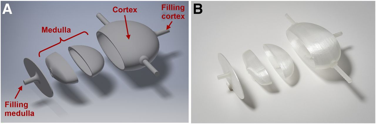
Division of kidney into 4 separate parts to enable fused deposition modeling 3D printing. (A) CAD model. (B) Printed parts.
Model-Based Calculation of Geometry-Specific Recovery Coefficients
For negligible background (i.e., no spill-in), the proportion of counts lost because of partial-volume errors can be analytically calculated as the ratio between the counts detected in a VOI precisely following the contours of the object ( ) and the counts initially originating in the object (
 ) (22):
 Eq. 3In other words,
  is a factor by which the number of counts in the VOI is lowered due to spill-out, often referred to as the recovery coefficient. The index g–s was added to indicate that
  , in contrast to the frequently applied sphere-based recovery coefficients, is geometry-specific. The partial-volume–corrected activity can be obtained by inserting Equation 3 into Equation 1:
 Eq. 4If the contour of the hot object is known (e.g., a CT-based object mask),
  can be determined as follows. First, SPECT imaging is simulated by convolving the high-resolution object mask with a gaussian kernel (Eq. 2 with predetermined FWHM) and resampling the resulting matrix to a grid of SPECT dimensions. Next, the volume of the object (Vobject) is divided by the volume of 1 SPECT voxel (Vvoxel) to obtain the number of SPECT voxels (
 ) that the object consists of:
 Eq. 5If the total intensity is normalized to 1,
  can then be approximated by adding up the
  voxels of maximum intensity:
 Eq. 6
Eq. 6
Comparison of Different Partial-Volume Correction Methods
SPECT/CT acquisitions were performed with the 177Lu-filled sphere, ellipsoid, and 2-compartment kidney (specific activity, 1.25 MBq/mL; ∼1.0 M total counts in the main energy window) separately mounted in the water-filled NEMA IEC body phantom (L981602; PTW-Freiburg). For the kidney, only the cortical compartment was filled with activity; the medullary compartment was filled with water.
After reconstruction, the activities were quantified by a VOI analysis in syngo.via (Siemens Healthineers). In the xSPECT case, the mean activity concentration was multiplied by the volume, and the cross-calibration factor to the dose calibrator was applied to obtain the activity. For Flash3D, the counts were converted to activity according to Equation 1. Finally, the following 5 methods for postreconstruction PVC were applied.
Method 1: CAD-Based Recovery Coefficient
First, a geometry-specific recovery coefficient  was calculated as described in the previous section (highly resolved mask: CAD design of the respective model, resolution from hot-sphere–cold-background experiment). Next, an isocontour VOI was drawn in the SPECT images with a volume exactly matching the filling volume extracted from the CAD model. Finally, the activity in the VOI was divided by
  to obtain the corrected activity (Eq. 4).
Method 2: CT-Based Recovery Coefficient
Like the CAD-based recovery coefficient method, the CT-based recovery coefficient method applied a geometry-specific recovery coefficient  for PVC. To mimic a realistic situation in which the contour of the scanned object is unknown before the acquisition, the highly resolved mask and the filling volume were extracted from the low-dose CT using 3D Slicer (Fig. 2B) (31).

Cross-section through kidney phantom at different stages. (A) CAD model. (B) CT-based segmentation in 3D Slicer. (C) Fused SPECT/CT reconstruction.
Method 3: Enlarged VOI
Isocontour VOIs (xSPECT, >50 kBq/mL; Flash3D, >200 counts) with volumes larger than the underlying object were drawn to account for spill-out.
Method 4: Peak Milliliter
A constant activity concentration was presumed in the entire object of interest. It was approximated by the activity concentration in the milliliter of the highest intensity and multiplied by the CT-based volume to estimate the total activity.
Method 5: 42% Fixed Threshold
In this simple yet widespread approach (32), a fixed threshold value of 42% of the maximum voxel value was applied to a large ellipsoidal initialization VOI containing the entire object as well as all potentially spilled-out counts. Finally, the threshold of an isocontour was varied between 1% and 40% to find an optimal threshold for SPECT-based activity determination.
Effect of Postreconstruction Filtering on Activity Determination
To examine the effect of gaussian postfiltering on the quantitative accuracy, reconstructions indicated as “standard” in the reconstruction software (xSPECT/Flash3D: 16/30 iterations, 1/2 subsets, 20.8-mm 3D gaussian filter) were additionally performed for all geometries. For a visual analysis, the same postprocessing filter was applied to the initial reconstructions of the sphere and kidney phantom.
RESULTS
Determination of Resolution
The resolutions determined in the hot-sphere–cold-background experiment are given in Table 2.
Determined Resolutions
Comparison of PVCs
Figure 2 shows the CAD model, the CT-based segmentation in 3D Slicer, and the fused SPECT/CT reconstruction of the renal cortex. The calculated recovery coefficients  are listed in Table 3. Although
  of sphere and ellipsoid differed by only −0.7% (mean over all reconstructions), a mean difference of −31.7% was found between sphere and renal cortex.
Geometry-Specific Recovery Coefficients 
The results of the activity determination are depicted in Figure 3. The quantification error (denoted as ΔxSPECT or ΔFlash3D) stands for the percentage difference between experimental (quantitative SPECT) and true (dose calibrator) activities. Moreover, the term |μΔxSPECT/Flash3D| describes the mean error (absolute values) over all 3 objects for the respective reconstruction method. Without postfiltering (Figs. 3A and 3B), the calculated recovery coefficients (CAD- and CT-based) led to the smallest errors for both reconstructions (|μΔxSPECT| = 1.5%, |μΔFlash3D| = 10.3%), followed by the enlarged volume with a systematic underestimation of 8.5% (xSPECT) and 13.0% (Flash3D). Although the peak-milliliter method exhibited a high systematic overestimation for the sphere and the ellipsoid (|μΔxSPECT| = 23.4%, |μΔFlash3D| = 21.6%), it underestimated the activity by 5.7% (xSPECT) and 11.1% (Flash3D) for the cortical geometry. The 42% threshold always showed the highest error (|μΔxSPECT| = 32.3%, |μΔFlash3D| = 46.7%).
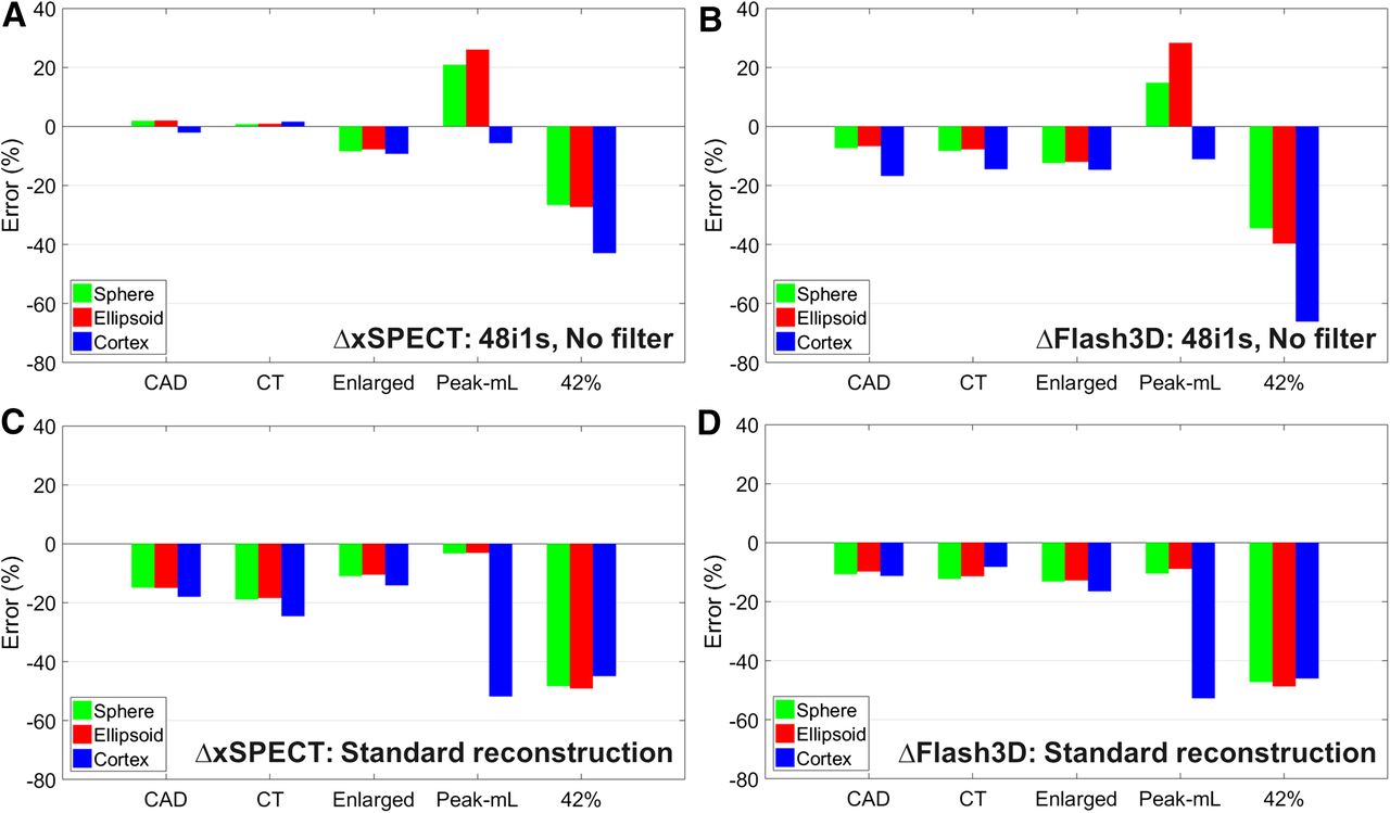
Accuracy of activity determination with different PVC methods. (A and B) xSPECT/Flash3D: 48 iterations, 1 subset, and no filter. (C and D) xSPECT/Flash3D standard reconstruction: 16/30 iterations, 1/2 subsets, and 20.8-mm gaussian filter.
The effect of gaussian postfiltering is illustrated in Figures 3C and 3D. For the filtered reconstructions, the activity was underestimated by all PVC methods. Two major changes were observed in comparison to the nonfiltered activity determination: first, the error of the geometry-specific recovery coefficients (methods 1 and 2) increased from 1.5% to 18.3% for xSPECT; second, the peak-milliliter error (method 4) decreased from 22.5% to 6.4% for the spheric and elliptic geometries, whereas it increased from 8.4% to 52.2% for the cortical geometry (average over both reconstructions).
The results of the optimum threshold experiment are given in Figure 4. For both unfiltered reconstructions, the difference between dose calibrator and SPECT/CT quantification decreased with the number of voxels included in the VOI. Although very small errors were reached for the smallest possible threshold of 1% (|μΔxSPECT| = 8.2%, |μΔFlash3D| = 11.4%), the activity always remained underestimated by the SPECT/CT quantification.
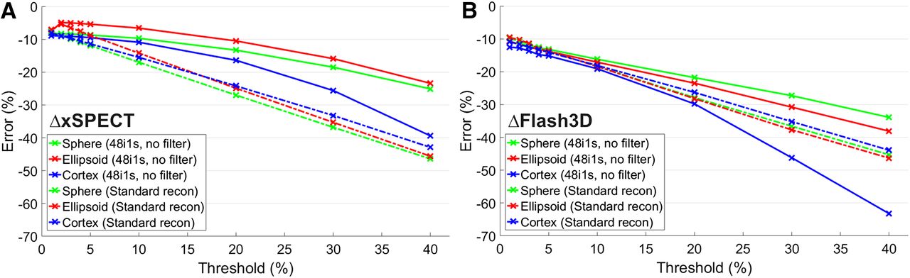
Threshold-dependent accuracy of activity determined with and without filtering for xSPECT (A) and Flash3D (B). Solid lines are for initial reconstruction (48 iterations, 1 subset, and no filter); dashed–dotted lines are for filtered standard reconstruction (xSPECT/Flash3D: 16/30 iterations, 1/2 subsets, and 20.8-mm gaussian filter).
The same behavior was observed for the filtered standard reconstruction, with minimum errors of |μΔxSPECT| = 7.7% and |μΔFlash3D| = 10.1% for a 1% threshold. Although there were differences between the cortex and both spherelike geometries in the unsmoothed case, these differences disappeared after the postfiltering.
DISCUSSION
Assessment of 3D Printing Technique
The kidney phantoms demonstrate the feasibility of manufacturing quasirealistic anthropomorphic phantoms with multiple, separately fillable compartments using low-cost 3D printing. Although the time-consuming processing chain (separate printing, support removal, coating, and agglutination) could, on the one hand, be accelerated by using more sophisticated 3D printing technology, considerably higher costs, on the other hand, would result. In combination with a comparably low purchase price in the lower 4-digit U.S. dollar range, the material costs of fused deposition modeling 3D printing are negligibly low even if high-quality filaments are used. As an example, about 50 g of filament were used for each of the kidneys (including support material), leading to costs of about 2 U.S. dollars per printed phantom, assuming a price of about 40 U.S. dollars per kilogram of high-quality filament.
Physical Phantom Versus Monte Carlo Simulation
When optimizing image quantification, verification of the results is of high importance. In principle, there are 2 options: physical measurements of objects with known activities, or Monte Carlo simulations of projection data. While the experimental methods suffer from a limited number of geometric objects that can be produced, Monte Carlo methods strongly depend on an accurate knowledge about the physical parameters of the γ-camera and the object to be simulated. Although many hardware specifications are available from the vendors (e.g., the material and geometry of the collimator), some proprietary information is not publicly available and has to be approximated (e.g., backscatter from material at the back of the crystal) (33). Although simulations can be optimized to include these poorly defined features, there always remains a difference between a physical phantom acquisition and the corresponding simulation. Although the focus of this work was the application of low-cost physical phantoms for the assessment of PVC methods in quantitative SPECT/CT imaging, the results of our measurements can easily be compared with Monte Carlo simulations, should they become available.
Assessment of PVCs
The geometry-specific recovery coefficients were found to be the best-performing means of postreconstruction PVC when background is negligible. Although method 1 relies on the CAD model of the examined object, which is available only in phantom acquisitions, method 2 obtains all necessary information from the low-dose CT scan, resulting in an equally efficient activity determination with errors of 1.0% (sphere), 1.1% (ellipsoid), and −3.7% (cortex). Therefore, the model-based recovery coefficients represent a promising PVC method for clinical SPECT/CT acquisitions. One of the major sources of error in this method lies in the handling of spatial resolution. In general, γ-cameras feature a distance-dependent spatial resolution. As the distance between the detector and the hot object is slightly changing between the views of any SPECT acquisition, the reconstructed SPECT images have a spatially varying and anisotropic resolution. Although this problem is addressed by most commercially available reconstruction algorithms, the resolution of the reconstructed images, to a certain degree, remains anisotropic and location-dependent. Although anisotropic and spatially varying point spread functions could be included in the model-based calculation of the recovery coefficients (Eq. 2), a constant spatial resolution was assumed across the phantom for simplicity, implemented by an isotropic and spatially invariant gaussian (9,22,34). Although the assumption of spatial invariance can be justified by the positioning of all phantoms in the center of the field of view, as well as the fact that the phantom dimensions (maximum, 11.4 cm) are about 6 times smaller than the useful field of view (61.4 cm), the assumption of isotropic resolution remains a source of error.
To demonstrate the propagation of resolution errors, geometry-specific recovery coefficients of varying FWHM (interval of [−2 mm, −1 mm, +1 mm, +2 mm] around the nominal value) were calculated (Table 4). A mean difference of 1.9%/3.6% occurs for a 1-mm resolution error, even increasing to 3.6%/9.0% for a 2-mm mismatch (sphere/cortex). Nevertheless, the geometry remains the dominating factor in the recovery coefficient calculation, with a difference of 31.7% between the spherelike objects (sphere, ellipsoid) and the more complex renal cortex. This is especially interesting as one of the most widespread approaches for PVC is based on volume-dependent recovery coefficients, which are based on sphere phantoms, but which are applied independently of the geometry in many applications.
Resolution-Dependency of Recovery Coefficients
A second major source of error lies in the delineation of the hot regions. In a clinical setting, the low quality and low resolution of the typically unenhanced low-dose CT acquisitions are often inadequate for reliable segmentation of the hot compartments. Although information from other imaging modalities such as MRI or full-dose CT could facilitate the delineation, insufficient knowledge about the ligand-specific radionuclide distribution inside typical organs of interest often impedes a morphology-based differentiation between hot and cold compartments.
If an accurate delineation should be impossible, method 3 represents an accurate and robust alternative for postreconstruction PVC without profound knowledge about the distribution of radiopharmaceutical inside the object of interest. Instead, spilled-out counts are simply included by an enlarged VOI.
Irrespective of the geometry, both maximum-intensity–based approaches led to considerable errors in the activity quantification, as can be partially explained by the fact that both methods take the maximum intensity in a small region as an estimate for the activity concentration in the entire VOI. In spherelike objects, the central voxels are far away from the object edges and, therefore, largely unaffected by partial-volume errors. In contrast, most voxels are close to one of the object edges in complex structures such as the renal cortex, causing these voxels to be affected by partial-volume errors. The result is a larger maximum intensity for sphere-shaped objects, causing the differences in the PVC (Figs. 3A and 3B). For the 42% threshold, the initial underestimation of 39.5% was reduced to 10.7% by reducing the threshold to 1% (Fig. 4). In this range, the method is equivalent to method 3, which includes essentially all spilled-out counts. In contrast, only the object volume can be changed for the peak-milliliter method, including yet another source of error.
As a final note, although the phantoms fabricated in this work demonstrate many aspects of the performance of the investigated PVC methods, many additional factors such as the object size, resolution, and noise level would have to be varied to justify a final assessment.
The Effect of Postreconstruction Filtering
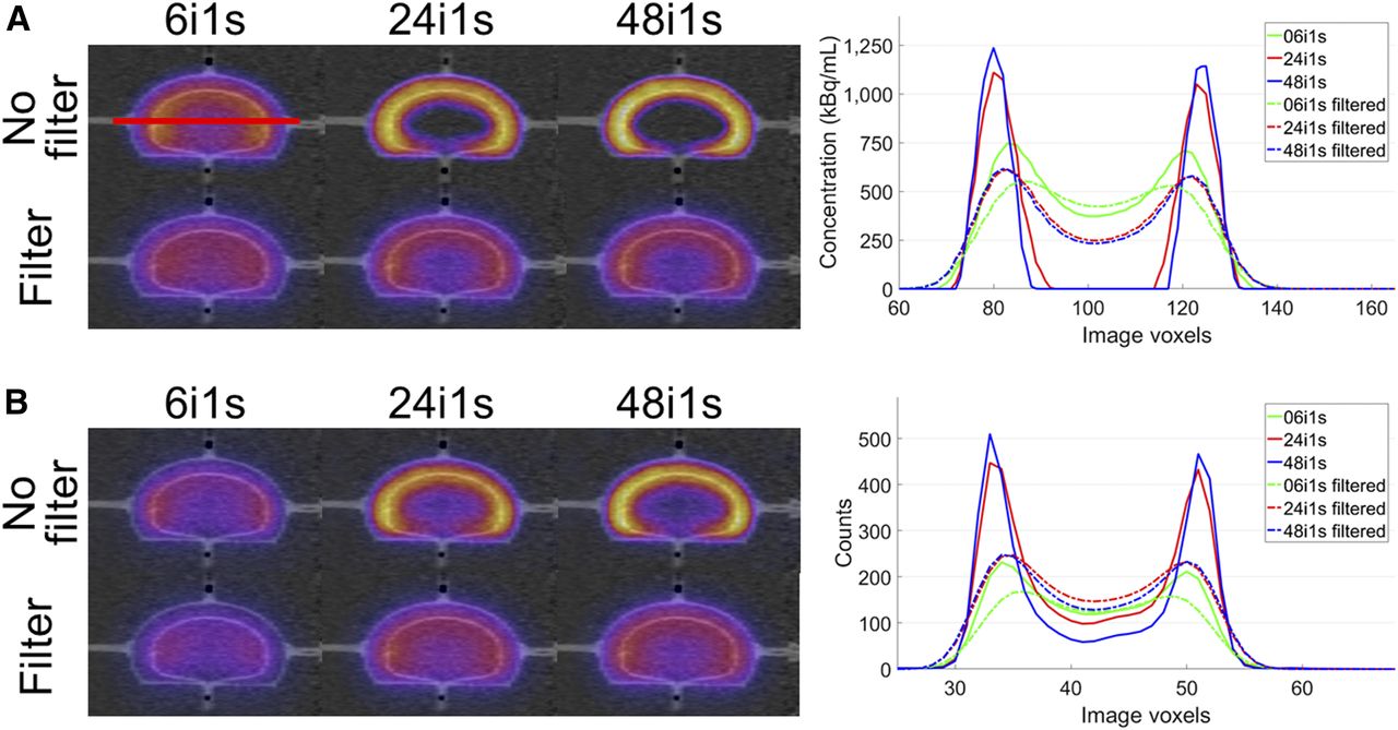
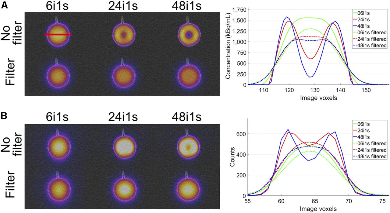
According to the quantification accuracy (Fig. 3), no postreconstruction filtering should be applied if postreconstruction PVC is to be performed. Lack of filtering can, however, lead to pronounced Gibbs ringing at the edges of larger objects such as the 100-mL sphere. To illustrate the evolution of this effect during the reconstruction, Figure 5 shows images of the sphere phantom and a cross-section for xSPECT and Flash3D at different stages of the reconstruction (6, 24, and 48 iterations) with and without postfiltering. Without the filter, Gibbs ringing occurs after a certain number of iterations (xSPECT, 24 iterations; Flash3D, 48 iterations). The more pronounced artifacts of the xSPECT reconstruction can be partly explained by the faster convergence of the underlying conjugate gradient minimization. Figure 5 shows that, for homogeneously filled objects, these artifacts can be effectively reduced by a gaussian filter. Unfortunately, the filters can lead to a blurred appearance of more complex structures, as is illustrated in Figure 6. Although the renal cortex is nicely resolved by the initial reconstruction, the postreconstruction filter makes the object appear to be almost homogeneously filled. Differentiation between unfiltered sphere and filtered renal cortex is almost impossible. Therefore, postreconstruction filtering should be applied cautiously.

Effect of gaussian postfiltering on sphere phantom for xSPECT (A) and Flash3D (B). Shown are fused SPECT/CT images at different stages of reconstruction (left) and horizontal cross-sections (right). Solid lines are for initial reconstruction; dashed–dotted lines are for filtered reconstruction.
Effect of gaussian postfiltering on kidney phantom for xSPECT (A) and Flash3D (B). Shown are fused SPECT/CT images at different stages of reconstruction (left) and horizontal cross-sections (right). Solid lines are for initial reconstruction; dashed–dotted lines are for filtered reconstruction.
Expanded Lookup Table for Geometry-Specific PVC
Volume-specific recovery coefficients, which are experimentally predetermined using spheric phantom inserts, are often used for PVC in oncologic applications. In this work, despite the similar filling volumes (∼100 mL), differences of 31.7% were found between the spheric and the renal geometry. These findings suggest that the sphere-based recovery coefficients should be replaced by a more geometry-specific solution in future applications. To cover various potential objects of interest, this novel lookup table could include basic geometries such as ellipsoids, toroids, and half-toroids of different proportions and volumes. By simulating the image formation (e.g., as presented in this work), geometry-specific recovery coefficients could be precalculated for a selection of typical resolutions. Depending on the shape of the object of interest and the SPECT/CT system used for the acquisition, a geometry- and resolution-specific PVC could then be applied for any SPECT/CT reconstruction without detailed studies as they are presented in this study. Experimental validation, however, will be extremely time-consuming and will, therefore, be subject to future work.
CONCLUSION
In this work, 3D printing was used as a prototyping technique for a geometry-specific investigation of SPECT/CT reconstruction parameters and PVC methods. A kidney phantom consisting of 2 separately fillable compartments was manufactured along with a sphere and an ellipsoid of the same volume. To investigate the efficiency of different PVC methods across various geometries, the accuracy of the SPECT/CT-based activity determination in kidney (hot cortex, cold medulla), sphere, and ellipsoid were compared. An unsmoothed SPECT/CT reconstruction in combination with a recovery coefficient based on the low-dose CT scan was found to be an optimal setup for activity determination. An average difference of 31.7% between spheric and renal recovery coefficients suggests that the typically applied recovery coefficient lookup tables, which are only volume-dependent, should be replaced by a more geometry-specific alternative.
DISCLOSURE
No potential conflict of interest relevant to this article was reported.
Footnotes
Published online Nov. 2, 2017.
- © 2018 by the Society of Nuclear Medicine and Molecular Imaging.
REFERENCES
- Received for publication August 1, 2017.
- Accepted for publication October 16, 2017.


Jump to section
Related Articles
Cited By...
- A Deep-Learning-Based Partial-Volume Correction Method for Quantitative 177Lu SPECT/CT Imaging
- A Pipeline for Automated Voxel Dosimetry: Application in Patients with Multi-SPECT/CT Imaging After 177Lu-Peptide Receptor Radionuclide Therapy
- Toward a Patient-Specific Traceable Quantification of SPECT/CT-Based Radiopharmaceutical Distributions
- What You See Is Not What You Get: On the Accuracy of Voxel-Based Dosimetry in Molecular Radiotherapy
- Characterization of Noise and Resolution for Quantitative 177Lu SPECT/CT with xSPECT Quant
- The Relevance of Dosimetry in Precision Medicine