


Abstract
Attenuation correction (AC) is a critical requirement for quantitative PET reconstruction. Accounting for bone information in the attenuation map (μ map) is of paramount importance for accurate brain PET quantification. However, to measure the signal from bone structures represents a challenging task in MR. Recent 18F-FDG PET/MR studies showed quantitative bias for the assessment of radiotracer concentration when bone was ignored. This work is focused on 18F-FDG PET/MR neurodegenerative dementing disorders. These are known to lead to specific patterns of 18F-FDG hypometabolism, mainly in superficial brain structures, which might suffer from attenuation artifacts and thus have immediate diagnostic consequences. A fully automatic method to estimate the μ map, including bone tissue using only MR information, is presented. Methods: The algorithm was based on a dual-echo ultrashort-echo-time MR imaging sequence to calculate the R2 map, from which the μ map was derived. The R2-based μ map was postprocessed to calculate an estimated distribution of the bone tissue. μ maps calculated from datasets of 9 patients were compared with their CT-based μ maps (μ mapCT) by determining the confusion matrix. Additionally, a region-of-interest comparison between reconstructed PET data, corrected using different μ maps, was performed. PET data were reconstructed using a Dixon-based μ map (μ mapDX) and a dual-echo ultrashort-echo-time–based μ map (μ mapUTE), which are both calculated by the scanner, and the R2-based μ map presented in this work was compared with reconstructed PET data using the μ mapCT as a reference. Results: Errors were approximately 20% higher using the μ mapDX and μ mapUTE for AC, compared with reconstructed PET data using the reference μ mapCT. However, PET AC using the R2-based μ map resulted, for all the patients and all the analyzed regions of interest, in a significant improvement, reducing the error to −5.8% to 2.5%. Conclusion: The proposed method successfully showed significantly reduced errors in quantification, compared with the μ mapDX and μ mapUTE, and therefore delivered more accurate PET image quantification for an improved diagnostic workup in dementia patients.
The current aging population is leading to an increased attention to dementing disorders and their most common cause, neurodegenerative Alzheimer disease. One of the earliest features seen on PET neuroimaging that these neuropsychiatric disorders show is reduced brain glucose metabolism in specific regions in neocortical brain areas. In addition to established biomarkers representing neuronal dysfunction such as 18F-FDG, newer protein aggregation PET biomarkers for in vivo amyloid imaging in the brain have been developed and were recently included into the guidelines of the National Institute on Aging and the Alzheimer Association (1,2). For all of these PET techniques, a highly accurate and robust tracer quantification is required for the early diagnosis and accurate monitoring of therapeutics such as amyloid-modifying agents.
A level of quantification error of below 5% for brain PET is desired (3). PET data require correction for scattering and attenuation before reconstruction. Scatter correction, estimated through either analytic or simulated models, is based on a previously estimated attenuation map (μ map).
Attenuation information is obtained through a CT scan in the case of PET/CT, which is then transformed from Hounsfield units to the corresponding linear attenuation coefficients (4). During the last few years, technologic advances on PET instrumentation have allowed the integration of clinical MR-compatible PET scanners (5,6). The combination of PET and MR information provides the opportunity of exploiting several new possibilities such as motion correction, combined PET and functional MR imaging, anatomically driven image reconstruction, or simultaneous functional–metabolic–anatomic acquisition among others. The benefits of these new possibilities are arguably dependent on their clinical application. In particular, for neurologic studies, the acquisition of a combined PET/MR scan for quasiperfect coregistration is required, which also provides patient comfort, reduced radiation exposure, and increased patient throughput because no PET/CT is necessary. However, the combination of PET/MR also brings several challenges that need to be addressed to obtain accurate quantitative information, 2 of them being attenuation correction (AC) and scatter correction.
The 2-point Dixon sequence is used in clinical routine to classify among 4 different tissues: background, fat, lungs, and soft tissue (7). For whole-body PET/MR, this approach provides errors of less than 10%, which are acceptable in the medical community, with the exception of bone lesions (8).
The particular case of brain PET is more demanding because the ratio between the amount of hard tissue (bone) and soft tissue is higher, thus potentially obtaining larger errors than in whole-body PET when bone is ignored in the μ map. In the particular case of brain PET studies, given the small structures present in the brain and the test–retest variability in PET quantification (3), the desired quantitative error should be lower than the error acceptable for whole-body PET.
There are studies that indicate that using the Dixon-based AC, ignoring bones in the μ map, produces significantly high quantitative errors, compared with CT-based AC (9,10). Other studies have looked at the error in different areas of the brain, proving that the largest quantitative errors are located near bone structures (11), the worst scenario being when bone is classified as air, for which errors up to 30% have been measured.
There are various alternatives to produce accurate attenuation information from the head. The most extended method is based on computed atlases using MR and CT information from the same patients to classify data into different tissues (12–14). In a slightly different manner, these atlases have been used in combination with machine-learning algorithms (15–17) to provide more accurate results. A combination of segmentation and atlas using SPM8 (Statistical Parametric Mapping; Wellcome Trust Institute of Neurology) (18) to calculate the μ map was presented by Izquierdo-Garcia et al. (19).
Alternatively, different segmentation methods applied to different MR sequences, such as magnetization prepared rapid acquisition gradient echo (MPRAGE) (20), ultrashort echo time (UTE) (21), or dual-echo UTE (dUTE) (22–24), have obtained accurate quantitative results. The latter represents an interesting approach because a preliminary good estimate of the μ map can be obtained using information extracted at different echo times (TEs). In all these methods, predetermined attenuation coefficients are assigned to each voxel depending on the assigned tissue, which can be air, soft tissue, fat, and bone. A detailed comparison of the approach introduced by Keereman et al. (23) with CT data was recently presented in Delso et al. (25). This study concluded that the μ map calculated by Keereman et al. (23) was a reliable method to extract the cortical bone but without a functional relation with CT data. However, artifacts were observed around dental implants, air interfaces, and nasopharyngeal cavities and within the folds of the neck fat. The analysis was limited to μ maps without presenting results from reconstructed PET data.
A third methodology uses attenuation information estimation from emission data, which has been investigated with the maximum-likelihood activity and attenuation algorithm (26). Moreover, some improvements were obtained by including time-of-flight information (27), reducing artifacts produced by cross-talk between emission and attenuation data. However, studies using this approach have been limited to whole-body studies, missing potential improvements particularly for brain PET studies.
In this work, we present a method to extract the head μ map calculated from a dUTE sequence, which is postprocessed to produce a continuous spectrum of linear attenuation coefficients. The method is similar to the one presented by Keereman et al. (23) but with higher emphasis on the image-processing approach to obtain the final μ map. Additionally, in our work we performed a quantitative analysis of dementia-related brain regions from reconstructed PET data.
MATERIALS AND METHODS
PET/MR Device
The PET/MR scanner used in this work was the Biograph mMR (Siemens AG-Healthcare) with the software version VB18SP3 and the work-in-progress software version 719. The mMR scanner is a fully integrated system with a 3-T MR magnet and a PET ring based on avalanche photodiode technology.
The dimensions of the magnet were a 163-cm outer diameter and 60-cm inner diameter with an axial field of view of 45 cm, and the dimensions of the PET bore were a 59.4-cm diameter with a 25.8-cm axial field of view.
The spatial resolution in the center of the scanner was 4.3 mm, and the sensitivity was 15 cps/MBq (28). The gradient coil had a gradient field of 45 mT/m, with a switching time of 200 T/m/s. The head/neck coil used in all the studies presented here was the 16-channel Total Imaging Matrix (Siemens AG-Healthcare).
Imaging Protocol
Nine patients (7 men and 2 women), with an average age of 61 ± 8 y (range, 51–76 y) and average weight of 82 ± 18 kg (range, 67–128 kg), were selected for the present prospective study. The patients, with suspected dementia, were selected for a double scan in the PET/CT system (Biograph mCT; Siemens AG-Healthcare) and subsequently in the PET/MR, which was located nearby. Patients were intravenously injected with 184 ± 6 MBq of 18F-FDG 30 min before the PET/CT scan, following the standard protocol in dementia studies. The head PET/CT scan took 15 min. A low-dose CT (120 keV, 25 mAs) scan was acquired for attenuation and scatter correction in the PET/CT. All subjects gave written informed consent, and the local Institutional Review Board approved the study.
After the PET/CT scan, the subjects immediately underwent a PET/MR scan without extra 18F-FDG administered. The tracer activity in the subjects when the PET scan started in the PET/MR was 138 ± 21 MBq. The duration of the PET scan in the PET/MR was 15 min. These emission data were used for reconstruction in combination with all the different μ maps studied in this work for each patient, including the CT-based μ map; hence, no decay correction was required and no physiologic discrepancies were present.
At the start of the MR protocol for neurologic studies, a dUTE sequence, which requires 100 s, was acquired. The dUTE consisted of 2 measurements taken at 2 consecutive TEs, 70 μs and 2.36 ms. The flip angle was 10° and the repetition time 3.98 ms. The field of view was 300 × 300 × 300 mm, with an isotropic voxel size of 1.56 mm. After the dUTE sequence, the rest of the sequences routinely used for dementia studies were acquired, extending the entire PET/MR scan for approximately 1 h.
Image Processing
The mMR system calculates 2 different μ maps for head AC. The routinely used μ map is based on the 2-point Dixon pulse sequence (μ mapDX), as used for whole-body AC, for which the head is classified as soft tissue and air cavities. Additionally, the mMR system also calculates a μ map based on a dUTE sequence (μ mapUTE), for which bone, soft tissue, and air cavities are identified. The way μ mapUTE is calculated is not disclosed by the vendor, but it is clear that it is computed by some relation between the resulting images obtained after both TE and posterior thresholding.
For comparison purposes, the CT data from the mCT was converted to μ map (μ mapCT) and used in the PET reconstruction for AC. To convert the CT data to μ values, the CT data in Hounsfield units were converted to linear attenuation coefficients for a 511-keV energy using a bilinear scaling (4). The resulting μ mapCT was then rigidly registered and resampled with the image acquired after the first echo obtained from the scanner using the Siemens Syngo 3-dimensional software to match the voxel size of both datasets.
PET data were reconstructed using the statistical iterative ordered-subsets expectation maximization (29), with 21 subsets and 3 iterations. The reconstructed field of view was 128 × 128 × 74 voxels, with a size of 2.54 × 2.54 × 3 mm. The images were filtered by a 5-mm-wide Hamming window after reconstruction.
Attenuation Map Estimation
The μ map used in this work was estimated as follows: at the start of each scan, a dUTE pulse sequence was acquired as described in the “Image Processing” section. The process is described in the flowchart shown in Figure 1 and detailed below.
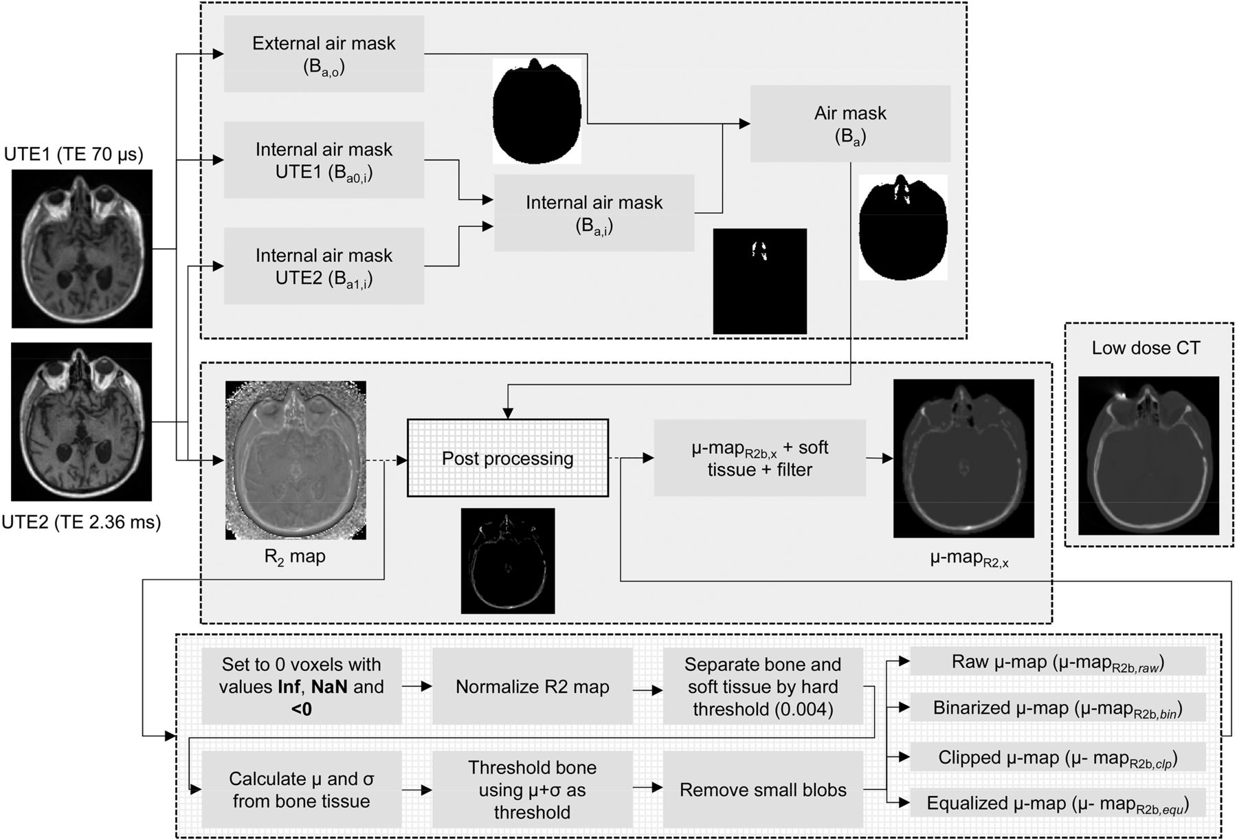
Flowchart to calculate μ mapR2,x.
Air Cavities
To identify the internal air cavities in the images measured after each echo, first the external region of the head was identified using a global histogram-based thresholding. The threshold value was automatically extracted from the valley of the resulting bimodal intensity histogram calculated from the first echo image, by calculating the intensity bin with the lowest gradient between histogram bins. After thresholding, the resulting external mask was defined as the outer air binary mask (Ba,o), where voxels identified as air were set to 1 and the rest were set to 0. The resulting Ba,o obtained from the first echo image was applied to both echo images. To find out the range of intensity values that each echo image contains corresponding to the internal air cavities, the mean (μBa,o) and SD (σBa,o) of the voxels included in the Ba,o mask were calculated in each echo image.
To extract the internal air cavities, all the voxels with intensity values less than μBa,o + σBa,o in each echo image were classified as air to produce the binary masks Ba0,i and Ba1,i for each echo image, respectively. Subsequently, the air cavities present in both air masks (Ba0,i and Ba1,i) were combined in a global internal binary mask (Ba,i) and merged with Ba,o to produce the global air binary mask (Ba).
Bone Tissue
To extract the bone tissue, the following relationship between the 2 images acquired after each echo was calculated: Eq. 1R2 is the inverse of the spin–spin transverse relaxation time (T2) from which the μ map is derived (23), where I1 and I0 are the resulting echo images and TE1 and TE0 are the echo times, 70 μs and 2.36 ms, respectively. A thorough comparison between the R2-based μ map and μ mapCT showed significant qualitative resemblance between both μ maps (25).
The idea behind the R2 map is that the first echo picks up signal from bone and soft tissue, whereas the second echo picks up signal only from soft tissue. The R2 map contains high-intensity values where bone tissue is located and low-intensity values for the rest of the tissues. There are additional tissues with short T2, such as facial and neck musculature, which are visible in the R2 map (25). To study the impact of possible variability between echo images, we obtained 12 scans of the same healthy subject at the beginning of the day and at the end of the day during several consecutive days. All the resulting echo images were coregistered using SPM8. The R2 map of each scan was calculated to see the impact of the interscan voxel variability on the R2 map.
R2 Map Postprocessing
After the R2 map was calculated, it was postprocessed to obtain an accurate estimation of the bone structures. First, the air mask was subtracted from the R2 map. Subsequently, the bone tissue was extracted from the R2 map to be scaled to linear attenuation coefficients. For this purpose, the R2 map was normalized so the maximum intensity value was 1. Subsequently, all the voxels with an intensity value greater than 0.004 (empirically chosen) were initially identified as bone tissue. From those voxels identified as bone tissue, the mode (Mb) and the SD (σb) were calculated. Then all the voxels in the R2 map with an intensity value greater than Mb + σb were identified as bone. Small differences were observed with 2σb and 3σb thresholds. The resulting mask was cleaned by discarding blobs with an area smaller than 5 voxels in each 2-dimensional slice, producing a μ map containing only bone tissue (μ mapR2b).
One of the potential problems of using the μ mapR2b is that the intensity values exhibit significant intensity variations, compared with the μ mapCT (25). To correct for the different intensity value ranges observed between CT and MR data, 4 methods to postprocess the intensity values of μ mapR2b were compared: μ mapR2b with intensity values resulting from Equation 1 (μ mapR2b,raw), μ mapR2b with intensity values clipped at a maximum value of 0.251 cm−1 obtained experimentally from CT data (μ mapR2b,clp), binary maps for which voxels classified as bone were set to 0.151 cm−1 (μ mapR2b,bin), and μ mapR2b with intensity values equalized (μ mapR2b,equ) using the equation Eq. 2where
  and
and  are the intensity values for the R2-based μ map and μ mapR2b,equ, respectively, with voxel index I;
  is the minimum intensity value of the μ map (R2 or CT) from all voxels with an intensity value above 0; and
  is the difference between the maximum- and minimum-intensity values of the μ map.
Finally, μ mapR2b,x was completed by including the soft tissue as a constant (0.096 cm−1) and filtered with a gaussian mask of 4.3 mm in full width at half maximum (28) to match the spatial resolution of the PET scanner to produce the final μ mapR2,x.
The algorithm presented here is fully automatic, takes approximately 5 s to compute in average, and is implemented in MATLAB (version 8.1; The MathWorks Inc.).
Quantitative Comparison
The different μ mapsR2,x were quantitatively compared with the μ mapCT, μ mapDX, and μ mapUTE from the same patients. The μ mapsR2,x, μ mapDX, and μ mapUTE were in a common coordinate system, but the μ mapCT had to be rigidly registered to the rest of the μ maps to have all the μ maps in the same coordinate system. To classify air, soft tissue, and bone in the reference μ mapCT the thresholds −200 and 700 HU were used. The global percentage of true-positives and false-negatives between the μ maps obtained from each method was calculated (confusion matrix) using the classes derived from the segmentation. Special attention was paid in the case of air classified as bone or vice versa, because such a misclassification could potentially produce significant errors in the reconstructed PET data.
For dementia studies, the most relevant/interesting regions are those of the neocortex such as the hippocampus, parietal (inferior and superior), temporal (inferior, middle, and superior), and frontal regions. The precuneus and posterior cingulate regions, especially, are the most typically affected regions in Alzheimer disease 18F-FDG and amyloid PET studies (30–32). The orbitofrontal cortex region was included in the analysis because of its proximity to bone and air cavities.
Reconstructed PET data obtained with the μ mapR2,raw, μ mapR2,bin, μ mapR2,clp, μ mapR2,equ, μ mapDX, and μ mapUTE were quantitatively compared with reconstructed PET data corrected using the μ mapCT.
To compare the different methods, all the reconstructed PET images were analyzed using SPM8. First, the MPRAGE dataset of each patient was rigidly registered to the common coordinate space of the μ maps and PET using the aforementioned same transformation. Then, the T1 (MPRAGE) Montreal Neurologic Institute (MNI) template was elastically registered to the MPRAGE dataset of each patient. The MNI template contains a voxel atlas holding 116 anatomic predefined regions based on the automated anatomic labeling atlas. Once the MNI template was in the same coordinate space as the MPRAGE data, it was used to extract the quantitative information from the PET data. Finally, the mean was extracted from all the 116 anatomic predefined regions. The figure of merit used for the comparison between methods was the normalized error (En), defined as Eq. 3using the μ mapCT–corrected PET images as reference. ĀCT and ĀX are the mean activities measured in a given region of interest (ROI) of the PET data reconstructed using the μ mapCT for AC and the alternative μ maps. Although SPM8 automatically analyzes the 116 anatomic predefined regions, we strictly concentrated on those regions related to different stages of dementia, especially those showing alterations in the early stages of dementia.
RESULTS
Robustness of dUTE Sequence
Figures 2A and 2B show a central axial slice of the mean and SD, respectively, for each voxel of the R2 map calculated from each scan. The logarithm of the coefficient of variation (CV defined as σ/μ) was additionally calculated (Fig. 2C). The CV exhibits high variability due to similar intensity values in I0 and I1 for voxels corresponding to tissues with long T2 and dissimilar intensity values in I0 and I1 for voxels with short T2 relaxation time. Because of the logarithms of I0 and I1 used in Equation 1, the differences obtained in the CV are enhanced. The mean and SD of the voxels belonging to bone, air cavities, and soft tissue in Figures 2A, 2B, and 2C, respectively, are shown in Supplemental Table 1 (supplemental materials are available at http://jnm.snmjournals.org).

Mean (A) and SD (B) for each voxel of R2 map calculated from each of 12 dUTE scans and log (CV) (C) measured from A and B.
Attenuation Maps
Figure 3 shows a 3-dimensional rendering of μ mapCT and μ mapR2b,equ of a patient. The central axial slice of the μ mapCT, μ mapR2,equ, and μ mapUTE are shown in Figures 3C, 3D, and 3E, respectively. The errors of μ mapR2,equ and μ mapUTE, compared with μ mapCT, are shown in Supplemental Figure 1.
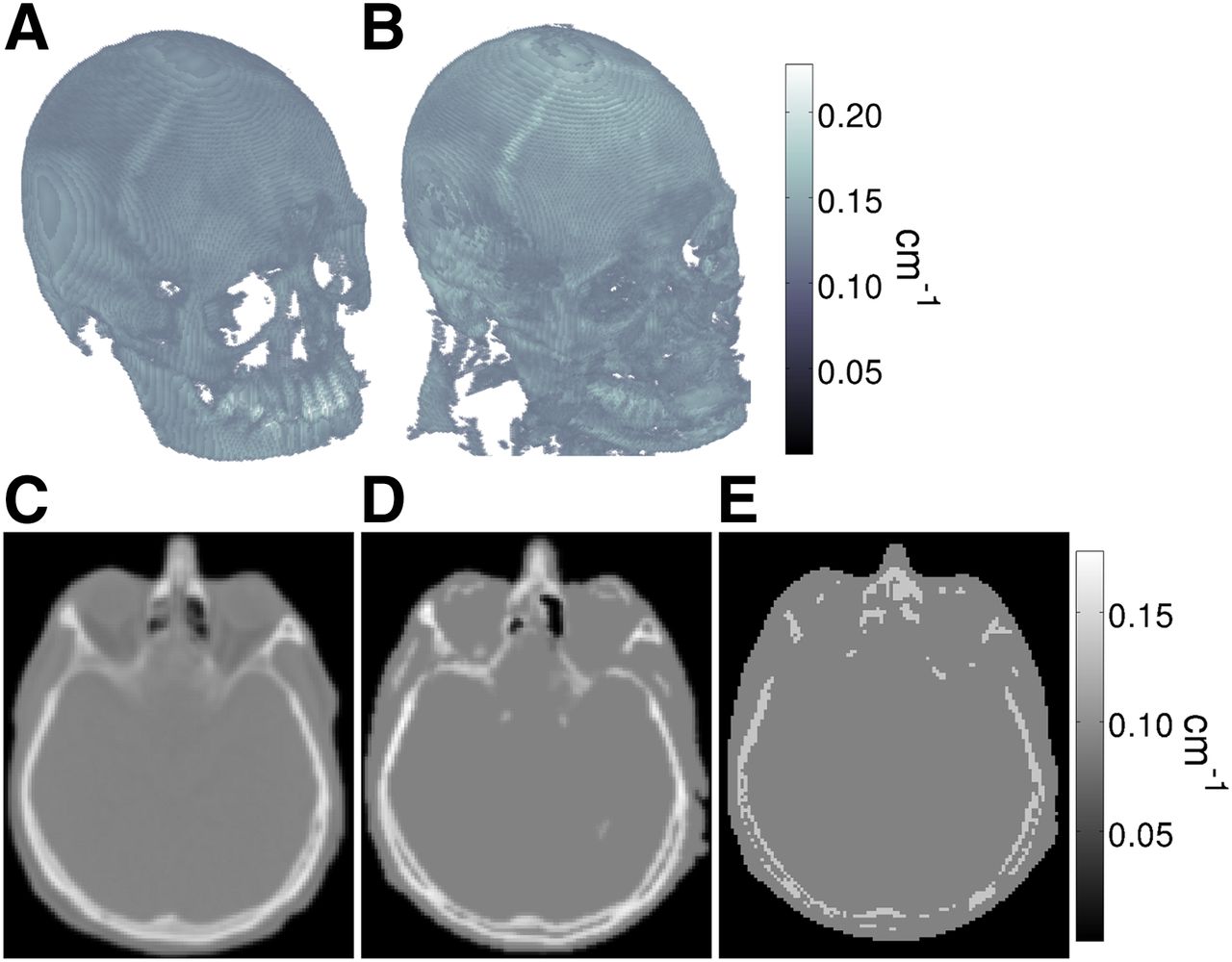
Three-dimensional rendering of bone structure of μ mapCT (A) and μ mapR2b,equ (B) of patient. Corresponding central axial slices of μ mapCT (C), μ mapR2,equ (D), and μ mapUTE (E) including air cavities and soft tissue.
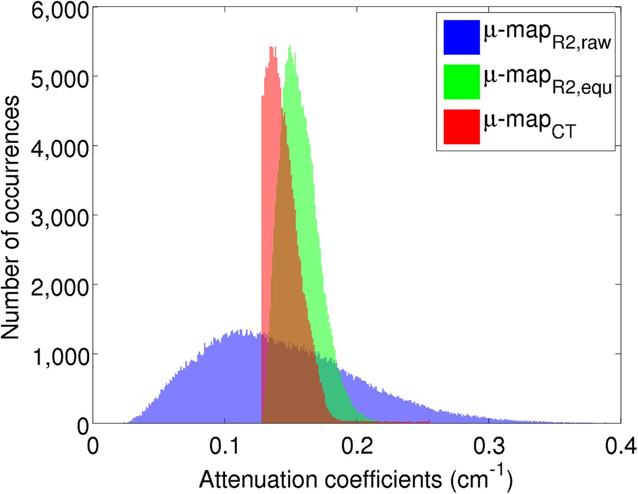
When the μ mapCT from all the patients was analyzed, the mode was 0.11 ± 0.00004 cm−1, the maximum value was 0.25 ± 0.009 cm−1, and the range (ΔICT) was 0.14 ± 0.009 cm−1. The low deviations suggest that the μ mapCT was consistent for all the patients. These parameters were used to equalize the μ mapR2b intensity values to match the CT attenuation coefficients. Figure 4 shows the intensity histograms of the bone structures from Figure 3, where the μ mapCT is shown in red, the μ mapR2b,raw in blue, and the μ mapR2b,equ in green.

Intensity histograms of voxels corresponding to bone from μ mapCT (red), MR from μ mapR2b,raw (blue), and μ mapR2b,equ (green).
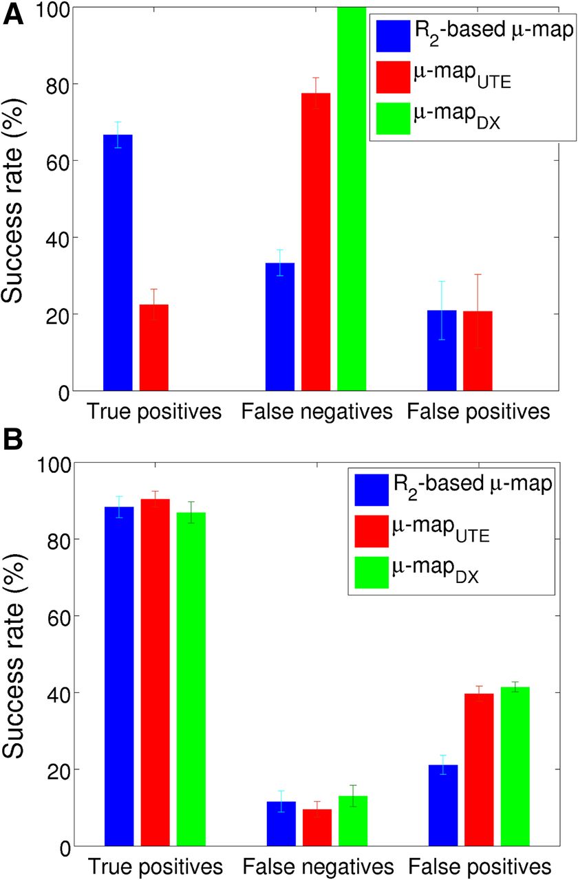
Figure 5A shows the classification results for bone and Figure 5B air using the μ mapCT as reference for the 3 different μ maps under evaluation: R2-based μ map, μ mapDX, and μ mapUTE (numeric values are in Supplemental Tables 2 and 3). True-positives represent the percentage of correctly classified voxels as bone or air. False-negatives correspond to the percentage of voxels belonging to bone or air incorrectly classified as a different tissue. Finally, false-positives correspond to the percentage of incorrectly classified voxels as bone or air, but they belong to a different tissue.

Percentage of classification success for bone (A) and air (B) for R2-based μ map (blue), μ mapDX (green), and μ mapUTE (red).
Considered a special case was when bone was classified as air or vice versa. The results for each method in the case for which voxels belonging to bone were misclassified as air and vice versa are shown in Supplemental Table 4.
Quantitative Comparison with Reconstructed PET Data
Figure 6 shows the En measured for the different ROIs related to dementia analyzed in this study. The μ maps used in each reconstruction were the μ mapDX and μ mapUTE calculated by the scanner and then the 4 alternatives based on the R2 map μ map: μ mapR2,raw, μ mapR2,bin, μ mapR2,clp, and μ mapR2,equ. The uncertainties, shown as error bars, were measured as the SD over the left and right hemispheres among all the patients. The numeric values of Figure 6A are shown in Supplemental Table 5. Supplemental Figure 2 shows central axial, coronal, and sagittal slices of the En for a patient using all the μ maps under study.
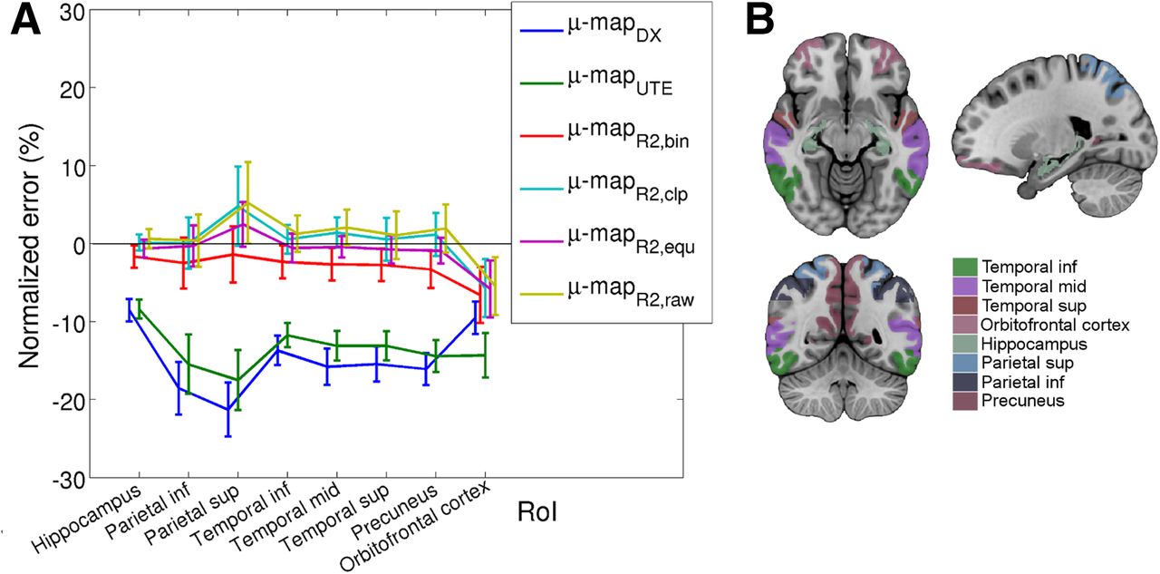
En for dementia-related ROIs (A) and analyzed ROIs (B) using μ mapUTE–based AC, μ mapDX–based AC, and μ mapR2,x–based AC with different postprocessing alternatives (μ mapR2,bin, μ mapR2,clp, μ mapR2,equ, and μ mapR2,raw). inf = inferior; mid = middle; sup = superior.
DISCUSSION
A variability study of the dUTE sequence resulted in higher variability in bone structures than soft tissues, which translates into higher variability in tissues with short T2 relaxation times than in tissues with long relaxation times. Such variability was additionally assessed in the R2 map by calculating the mean and SD for each voxel between the 12 scans. To see if the variability was significant, the log(CV) was calculated to study the noise. This calculation showed low CV in bones, compared with soft tissues, suggesting that using the R2 map to estimate the bone structures produces reliable results.
As indicated by other authors, the main challenge in estimating the μ map is to separate bone and air cavities (33), especially in regions in which they are close together (34) and tissue misclassification can result in significant errors.
The assessment of the tissue classification showed that our method performed better than the μ mapUTE, not only at correctly identifying voxels as bone (66.6%, compared with 22.4%) but also at misclassifying fewer voxels of bone as soft tissue (33.3%, compared with 77.5%).
Regarding the air cavities, the 3 methods performed similarly at correctly classifying voxels as air (88.6% ± 2.5% accurate) and misclassifying voxels of air as another tissue (11.4% ± 2.5% misclassified). However, the proposed method misclassified fewer voxels as air that actually belonged to another tissue (21.2% ± 2.5%, compared with 41.5% ± 1.3%), concluding that the other 2 methods significantly overclassified voxels as air.
In the special case in which air and bone can be interchangeably misclassified, the proposed method produced lower errors than the other methods at classifying voxels of bone as air (1.7%, compared with 2.7% and 5.2%). However, the proposed method produced a slightly higher error (3.6%, compared with 0.9%) than the other methods classifying voxels of air as bone. This was attributed to the low number of voxels classified as bone (0% in the case of μ mapDX) for the μ mapUTE.
μ mapR2,equ uses patient-specific CT minimum and maximum values for equalization; however, we observed negligible variations among our patient population. Thus, the use of non–patient-specific values would be possible if a reference CT-based μ map is not available.
The quantification errors, obtained in the ROI analysis from reconstructed PET data using the μ mapDX, were consistently the highest (except for the orbitofrontal cortex), compared with the other μ maps. These high values were attributed to the total absence of bone. The mean En calculated between all the ROIs was −14.8% ± 3.9% (μ mapDX), −13.5% ± 2.5% (μ mapUTE), 0.88% ± 2.7% (μ mapR2,raw), 0.36% ± 2.6% (μ mapR2,clp), −2.90% ± 1.5% (μ mapR2,bin), and −0.87% ± 2.1% (μ mapR2,equ). Even though the mean En obtained with the μ mapR2,raw and μ mapR2,clp were comparable to the En obtained with the μ mapR2,equ, the reconstructed PET data showed in some cases tracer uptake that was not present in any of the other approaches. Therefore, these were considered as false-positives. Supplemental Figure 3 shows exemplary axial slices of reconstructed PET data using μ mapCT, μ mapR2,raw, μ mapR2,clip, μ mapR2,bin, and μ mapR2,equ, showing abnormal tracer uptake (indicated with an arrow) for the cases of μ mapR2,raw and μ mapR2,clip, compared with the other μ maps. In the specific case of dementia studies, in which the regions to analyze are well defined, these false-positives may not represent a problem. However, in the case of extending this approach to oncologic studies, the false-positives represent a limitation to this algorithm. Consequently, the μ mapR2,raw and μ mapR2,clp were not further considered as reliable approaches for future studies. The worst performance in the ROI analysis was obtained with the μ mapR2,bin, which showed that a continuous spectrum of attenuation coefficients is more suitable than using discrete attenuation coefficients, as used in other works (11,14,16,23,24).
Clipping the attenuation coefficients from the μ mapR2b (μ mapR2,clp) provided the minimum mean En. However, these results must be assessed individually per ROIs, because the differences observed between the different μ mapsR2,x were too low and a global value is not meaningful.
From a diagnostic point of view, the hippocampus, which is a region close to dense bone, resulted in a mean En above −2%. The lowest error was obtained with the μ mapR2,clp (0.1%) and the highest with the μ mapR2,bin (−1.6%).
The orbitofrontal cortex is another dementia-related brain region that was included in the analysis because of its location in a region in which bone and air cavities are next to each other. Thus, tissue misclassification would exacerbate the quantitative difference. Interestingly, this region was the only one that showed a change of tendency of all the ROIs included in the analysis when comparing between μ mapDX and μ mapUTE. This effect was attributed to the classification of voxels in the air cavities as bone. This ROI also showed the highest En among all the analyzed ROIs for all the methods based on the R2-based μ map, the highest En being for the μ mapR2,bin (−6.6%) and the other methods showing similar results (−5%).
The parietal superior area also showed a remarkably high En, compared with the rest of ROIs. The reconstructed PET data using the μ mapDX and μ mapUTE showed the highest En, −21.2% and −17.5%, respectively, whereas the En dropped down to 2.45% with the μ mapR2,equ.
The rest of the ROIs showed homogeneous En for each μ map. The measured En average among the rest of the ROIs was −15.9% ± 1.7% (μ mapDX), −13.5% ± 1.4% (μ mapUTE), 1.3% ± 0.6% (μ mapR2,raw), −2.7% ± 0.3% (μ mapR2,bin), 0.7% ± 0.5% (μ mapR2,clp), and −0.5% ± 0.2% (μ mapR2,equ).
To put these results in perspective, compared with other approaches for which the error was measured in the same way as in this study, mean global errors of −5% and maximum errors of approximately −20% to 40% were obtained in structures near bone, especially those close to air cavities (23,24). More successful approaches obtained mean errors of 0.2% (12), 2.40% (17), and 2.74% (19) using ROI analysis. However, these methods rely on databases (MPRAGE, CT, Dixon-volume interpolated breath-hold examination, UTE) that are not always available; require a training process (17), which has an impact on the classification performance; and have a computation time of 7–30 min to calculate the μ map.
All the aforementioned works used a μ mapCT as a reference. The use of μ mapCT for AC as reference is recognized as the gold standard. However, there is some doubt about the reliability of CT for absolute quantitation (35). Studies to confirm the accuracy of CT-based AC and MR-based AC using phantoms, for which the amount and density of attenuating material are known, are ongoing.
CONCLUSION
In this work, we compared the μ map based on the R2 map with the μ maps calculated by the mMR scanner, the μ mapDX and μ mapUTE. The comparison was performed at 2 levels: first by analyzing the rate of correctly classified bone and air in each μ map and second by comparing the activity concentration measured in regions related to dementia obtained after reconstructing the PET data, using the different μ maps for AC.
Results showed that the R2-based μ map, independent of the postprocessing method, produced more accurate quantitative information than the μ mapDX and μ mapUTE. The worst results were consistently obtained with the μ mapDX with PET quantitative errors of 8%–21% depending on the ROI, whereas the μ mapUTE improved only by approximately 2% on average, compared with the μ mapDX.
The proposed method based on the μ mapR2,equ showed consistently better tissue classification and more accurate PET quantitative results than those obtained with the μ mapDX and μ mapUTE, reducing the PET quantitative error to −5.8% to 2.5%.
DISCLOSURE
The costs of publication of this article were defrayed in part by the payment of page charges. Therefore, and solely to indicate this fact, this article is hereby marked “advertisement” in accordance with 18 USC section 1734. The PET/MR facility at the Technische Universität München was funded by the Deutsche Forschungsgemeinschaft, Großgeräteinitiative (DFG). The research leading to these results has received funding from the European Union Seventh Framework Program (FP7) under grant agreement no. 294582 ERC Grant MUMI and grant agreement no. 602621 Grant Trimage and from the DFG grant no. FO 886/1-1. No other potential conflict of interest relevant to this article was reported.
Acknowledgments
We thank Sylvia Schachoff and Claudia Meisinger for their technical assistance with the PET/MR scanner.
Footnotes
↵* Contributed equally to this work.
Published online Feb. 12, 2015.
- © 2015 by the Society of Nuclear Medicine and Molecular Imaging, Inc.
REFERENCES
- Received for publication July 30, 2014.
- Accepted for publication January 12, 2015.


Jump to section
Related Articles
Cited By...
- Zero-Echo-Time and Dixon Deep Pseudo-CT (ZeDD CT): Direct Generation of Pseudo-CT Images for Pelvic PET/MRI Attenuation Correction Using Deep Convolutional Neural Networks with Multiparametric MRI
- The Effect of Susceptibility Artifacts Related to Metallic Implants on Adjacent-Lesion Assessment in Simultaneous TOF PET/MR
- Clinical Evaluation of Zero-Echo-Time Attenuation Correction for Brain 18F-FDG PET/MRI: Comparison with Atlas Attenuation Correction
- MRI-Based Attenuation Correction for PET/MRI Using Multiphase Level-Set Method