


Abstract
The serotonin (5-hydroxytryptamine, or 5-HT) type 1A receptor (5-HT1AR) is implicated in the pathophysiology of numerous neuropsychiatric disorders. We have published the initial evaluation and reproducibility in vivo of [O-methyl-11C]2-(4-(4-(2-methoxyphenyl)piperazin-1-yl)butyl)-4-methyl-1,2,4-triazine-3,5(2H,4H)dione (11C-CUMI-101), a novel 5-HT1A agonist radiotracer, in Papio anubis. Here, we report the optimal modeling parameters of 11C-CUMI-101 for human PET studies. Methods: PET scans were obtained for 7 adult human volunteers. 11C-CUMI-101 was injected as an intravenous bolus, and emission data were collected for 120 min in 3-dimensional mode. We evaluated 10 different models using metabolite-corrected arterial input functions or reference region approaches and several outcome measures. Results: When using binding potential (BPF = Bavail/KD [total available receptor concentration divided by the equilibrium dissociation constant]) as the outcome measure, the likelihood estimation in the graphical analysis (LEGA) model performed slightly better than the other methods evaluated at full scan duration. The average test–retest percentage difference was 9.90% ± 5.60%. When using BPND (BPND = fnd × Bavail/KD; BPND equals the product of BPF and fnd [free fraction in the nondisplaceable compartment]), the simplified reference tissue method (SRTM) achieved the lowest percentage difference and smallest bias when compared with nondisplaceable binding potential obtained from LEGA using the metabolite-corrected plasma input function (r2 = 0.99; slope = 0.92). The time–stability analysis indicates that a 120-min scan is sufficient for the stable estimation of outcome measures. Voxel results were comparable to region-of-interest–based analysis, with higher spatial resolution. Conclusion: On the basis of its measurable and stable free fraction, high affinity and selectivity, good blood–brain barrier permeability, and plasma and brain kinetics, 11C-CUMI-101 is suitable for the imaging of high-affinity 5-HT1A binding in humans.
The serotonergic system and the serotonin (5-hydroxytryptamine, or 5-HT) type 1A receptor (5-HT1AR) are implicated in psychiatric disorders and the action of antidepressants (1–8). Positron emission tomography (PET) radiotracers allow in vivo quantification of 5-HT1AR binding.
G-protein–coupled receptors exist in a high-agonist-affinity state that is bound to G-proteins and a low-affinity state (uncoupled from G-protein) (9,10). Antagonists bind to either state with equal affinity, and existing PET radiotracers for this receptor are antagonists. Additionally, agonist radiotracers are more likely to be sensitive to changes in intrasynaptic concentrations of the neurotransmitter (11), as demonstrated in the dopaminergic system (12). [O-methyl-11C]2-(4-(4-(2-methoxyphenyl)piperazin-1-yl)butyl)-4-methyl-1,2,4-triazine-3,5(2H,4H)dione (11C-CUMI-101), a new agonist radioligand (13), has a measurable free fraction and highly reproducible binding potential (BPF) in Papio anubis (14).
We evaluate several modeling methods for quantifying 11C-CUMI-101 binding in humans using a test–retest paradigm. We consider estimation of BPF (Bavail/KD [total available receptor concentration divided by the equilibrium dissociation constant]), the closest approximation to Bavail, at 6 different scanning durations.
MATERIALS AND METHODS
The study was approved by the Institutional Review Board, and participants gave written informed consent. Ten healthy volunteers signed an informed consent form, and 7 (3 women, 4 men; mean age ± SD, 32 ± 7 y) completed the study and were included in the analysis.
Radiochemistry
11C-CUMI-101 was synthesized as previously described (13,14). The chemical purity of 11C-CUMI-101 was 99.4% ± 2.3%, and the radiochemical purity was 99.4% ± 0.6%.
PET Studies
The PET procedure is described elsewhere (15–17). Polyurethane head molds minimized motion (Soule Medical). An ECAT HR+ scanner was used (Siemens/CTI). 11C-CUMI-101 was injected over 30 s (384.84 ± 137.12 MBq [10.4 ± 3.7 mCi], with a mean specific activity of 33.54 ± 10.36 GBq/mmol [0.91 ± 0.28 mCi/nmol]). The average injected mass was 4.26 ± 0.68 μg. Fourteen brain regions were evaluated. Correlations between injected mass and volume of distribution (VT) ranged from −0.21 to 0.38 (P values ranged from 0.18 to 0.92). Emission data were collected in 3-dimensional mode for 120 min using 21 frames of increasing duration (3 × 20 s, 3 × 1 min, 3 × 2 min, 2 × 5 min, 10 × 10 min).
Input Function Measurement
The measurement of input function has been described elsewhere (15–17). Briefly, arterial samples were collected every 10 s in the first 2 min and less frequently thereafter, centrifuged, and plasma-separated. After initial extraction, the percentage of 11C-CUMI-101 radioactivity in plasma was determined by high-performance liquid chromatography (13). These fractions were then plotted and fit with a Hill's function (18). The product of the unmetabolized fraction and the total plasma counts was fit with a second-order polynomial from time zero to the plasma peak and the sum of 3 exponentials from the peak to the end. The mean free fraction (16) was 0.30 ± 0.03.
Image Analysis
Using a 3-T Signa HDx system (GE Healthcare), we acquired T1-weighted MR images (3-dimensional fast spoiled gradient-recalled echo) for coregistration with PET images and identified regions of interest (ROIs) (17). Subject motion was corrected by coregistering each PET frame to frame 8, using FLIRT (FMRIB linear image registration tool, version 5.0; FMRIB Image Analysis Group). After attenuation correction, PET-to-MRI transformations were computed using FLIRT with a mutual information cost function and 6 degrees of freedom. Eight different coregistration possibilities, with varying source or target images and weighting masks, were performed, as previously described (19). The optimum transformation was applied to the average PET image and all PET frames. Images were resliced in FLIRT with trilinear interpolation, and the results were verified by visual inspection.
Automatic ROIs were obtained for all regions except the raphe, which was manually drawn on the subject's PET image. The algorithm assigns probabilistic ROIs to an MR image using an automated multilabel approach, in which the ROIs from each of 18 templates, after being gray-matter–masked, are nonlinearly transformed to the MR image. The 18 templates were created using 18 healthy subjects’ MRI brain scans. ROIs were hand-drawn on each template MR image by experienced technicians trained to reliably approximate these regions using brain atlases (20,21) and published reports (22,23). Before the templates were applied to study subjects, each subject's MR image was preprocessed with Freesurfer (http://surfer.nmr.mgh.harvard.edu/), and the bias-corrected and intensity-normalized results were used in conjunction with gray matter, white matter, and cerebrospinal fluid maps derived with SPM5 (Wellcome Department of Cognitive Neurology) to remove nonbrain areas. Each of the 18 template MR images was then nonlinearly registered with the Automated Registration Toolbox (24) to the target subject's brain (25). To calculate the probability of an ROI label for a particular voxel, the total number of transformed template ROIs assigned to that voxel was counted and divided by 18. Cortical regions were then gray-matter–masked using the target subject's segmentation. This masking was done for each ROI separately and for each voxel to establish a probabilistic set of ROIs in target subject space for use in PET analysis. For the 7 subjects, the average sizes (in cm3) of the automatically delineated regions, from largest to smallest, were 192.5 ± 14.7 (parietal lobe), 160.1 ± 12.7 (occipital lobe), 148.8 ± 14.2 (temporal lobe), 146.5 ± 7.0 (dorsolateral prefrontal cortex), 90.2 ± 5.8 (orbital prefrontal cortex), 63.8 ± 5.8 (cerebellar gray matter), 59.5 ± 4.0 (medial prefrontal cortex), 31.7 ± 2.5 (cingulate), 21.0 ± 1.4 (insula), 18.7 ± 1.5 (hippocampus), 17.1 ± 1.6 (entorhinal cortex), 11.6 ± 0.7 (posterior parahippocampal gyrus), and 10.6 ± 0.8 (amygdala). The VT derived from probabilistic ROIs used in this analysis was correlated with corresponding hand-drawn ROIs for 11C-WAY-100635 and 11C-DASB (n = 30; r2 > 0.98).
Modeling
Modeling approaches can be divided into 2 major categories: kinetic and graphical (14–17). The 2-tissue-compartment (2TC) kinetic model uses a standard iterative nonlinear least squares algorithm for constrained (where the ratio of K1/k2 is constrained to the value of the reference region's [RR's] VT) and unconstrained approaches. For the noniterative approach (26) (2TCNI), the time–activity curve is regressed on each of a library of functions. Likelihood estimation in graphical analysis (LEGA) (27,28) is a bias-free alternative to graphical analysis (29), using the last 8 time points for fitting. One-tissue-compartment and 3-tissue-compartment models proved to be unreliable and overparameterized and are not presented.
Three methods not requiring blood sampling were evaluated: the simplified reference tissue model (SRTM) (30) and bloodless versions of Logan analysis and LEGA. These methods used the gray matter of the cerebellum (CGM, obtained by applying an SPM5-derived gray-matter mask to the cerebellum) as an RR.
All modeling methods were applied to the time–activity curve data using a 5% blood volume correction. Weights (wi) were assigned to each frame according to
Six metrics were used to compare the models: percentage difference (PD) and within-subject mean sum of squares (WSMSS) for reproducibility, percentage SD (%SD) of BPF, intraclass correlation coefficient (ICC) for reliability, median absolute deviation of bootstrap resampled data for identifiability, and time stability (TS). Each of these has been described before (14–17), with the exception of %SD.
The %SD of an outcome measure is the SD of the sample (across experiments) divided by the sample mean.
For the RR techniques, the percentage bias was also calculated as (
Voxel-Level Analysis
VT parametric images were obtained by applying empirical Bayesian estimation in graphical analysis (EBEGA) (31), a fully automatic approach that incorporates LEGA (28) VT estimation in a Bayesian framework. The bloodless version of the Logan method was also considered for the generation of BPND parametric images.
RESULTS
The uptake of 11C-CUMI-101 is consistent with the known distribution of 5-HT1ARs (Fig. 1; Table 1).

11C-CUMI binding. (Top) MR images of subject. (Middle) Sum of last 60 min (6 frames) of PET acquisition. (Bottom) BPF value of every voxel within brain slices (calculated using EBEGA), with color bar indicating values of BPF data shown.
Metrics on High-Binding ROIs Using 120-Minute Scan and LEGA
Modeling
Figure 2 shows a representative hippocampal time–activity curve. 2TC methods fit the data well; iterative and noniterative 1-tissue-compartment models do not and are excluded from further analysis. Logan analysis and LEGA produce similar fits (Fig. 2, right).

Hippocampal time–activity curve fits. On left side, 2TC (iterative, 2TC; noniterative, 2TCNI; constrained, 2TCC) model fits are indicated. Raw data are shown with diamonds. On right side, raw data are shown (◆) transformed into space used for graphical interpretation. Cp is concentration of ligand in plasma, and CROI is concentration of ligand in hippocampus. 1TC = 1 tissue compartment; 1TC-NI = 1 tissue compartment, noniterative; SUV = standardized uptake value.
Although the measure of interest is Bavail, the closest measure of receptor density that can be estimated using PET is BPF (Bavail/KD), because 1/KD cannot be determined. Metric comparisons and TS analysis are performed on BPF.
Logan analysis and LEGA are the best performers in most metrics (Table 2).
Outcome Metrics Using 120-Minute Scan and BPF
Although LEGA performs slightly better than do the other methods, the outcome metric comparisons are not strongly sensitive to model choice. Most models tested perform similarly; metric results in a single category fall within 1 SD. For all high-binding ROIs (Table 1), when BPF estimated by 2TC methods is correlated with BPF estimated by the LEGA approach, the slopes are close to unity (1.02, 1.02, and 1.12 for the 2TC, constrained 2TC, and 2TCNI methods, respectively), with small intercepts (−0.29, 0.26, and −1.79, respectively) and R2 values greater than 0.90 (0.96, 0.99, and 0.95, respectively). Similar results were found when BPF estimated by Logan analysis was regressed against LEGA results (slope = 1.00; intercept = −0.35; R2 > 0.99).
For completeness, the comparisons performed in Table 2 were repeated using the ratio (at equilibrium) of specifically bound radioligand to that of total parent radioligand in plasma (BPP = fP * Bavail/KD) in Table 3. Though the metrics are different, the relative performance of each of the models is similar.
Outcome Metrics Using 120-Minute Scan and BPP
Table 2 shows average metrics across all subjects and all ROIs. However, Bavail, hence required scan duration, may vary with each ROI (Table 1).
Most ROIs achieve less than 10% difference between test and retest, on average, and the lower-binding ROIs generally attain lower WSMSS and lower average identifiability values than the higher-binding ROIs (Table 1).
Because both free fraction and binding in the RR will affect the estimation of BPF, outcome measures and metrics calculated using VT (Table 4) are presented.
Metrics on High-Binding ROIs Using 120-Minute Scan and LEGA
Rate constants are important for assessing ligand kinetics and are presented in Table 5.
Average and SD of Kinetic Rate Constants Using 120-Minute Scan and 2-TC Noniterative Method
Time Stability
TS was analyzed to determine the optimal scan duration. In aggregate, BPF was not stable before 110 min (Fig. 3).

BPF TS. BPF was calculated using 5 models at 6 scan durations. For each region, percentage of total scans (n = 14) in which calculated BPF was within 5% of BPF calculated at 120 min was determined. This plot shows average of these percentages over all regions tested. Error bars indicate SD. Constr = constrained.
In several ROIs, BPF values calculated using 110 min of scan data were within ±5% of those calculated using the full 120 min of data (Table 6). For other ROIs, 71% or more of the studies yielded stable BPF values at 110 min of scan time. The TS analysis was also repeated for VT. Except for 3 ROIs, VT values were stable at 110 min of scan time, suggesting that shorter scans may be possible, depending on the application and the target ROI. VT values converge faster than BPF values (Table 6). On average, VT values were within 8% of their terminal values from 70 min.
Time–Stability Analysis of High-Binding ROIs Using LEGA
RR Approaches
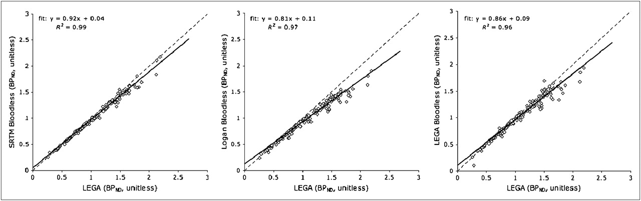
The 3 RR models produce BPND values lower than those from LEGA with a plasma input function (Fig. 4). Slopes of the regression lines predicting bloodless model outcomes from those calculated using LEGA with plasma input are 0.81, 0.86, and 0.92 for bloodless versions of Logan analysis and LEGA and SRTM, respectively. The intercepts range from 0.04 to 0.11.

LEGA BPND with plasma input, compared with BPND values calculated by RR approaches. All high-binding ROIs listed in Table 1 are included. Identity lines are plotted (dashed lines) for reference.
The mean PD over all high-binding ROIs yields similar results across RR approaches using BPND (Table 7). However, SRTM was the best performer in almost all metrics.
Metrics for Bloodless Models Using 120-Minute Scan and BPND
The TS was also analyzed using RR approaches. At 110 min of scan time, 95.05% ± 8.93% of the SRTM results were stable, on average. Bloodless Logan analysis and LEGA results at 110 min were both less than 80% stable. When SRTM BPND values at 110 min were regressed against BPND values calculated using LEGA and 120 min of scan time, the results were similar to those in Figure 4 (slope = 0.91, intercept = 0.05, and R2 = 0.99). Metric comparisons calculated using SRTM at 110 min did not vary greatly from those presented for SRTM (with 120 min) in Table 7 (9.98% ± 11.82%, 0.008 ± 0.003, 0.64 ± 0.16, 15.57% ± 5.60%, and −3.83% ± 4.56% for mean PD, WSMSS, ICC, percentage SD, and percentage bias, respectively).
Voxel Analysis
Modeling kinetic parameters on a voxel level, as opposed to an ROI level, provides greater spatial resolution. On an ROI level, LEGA has been proven to be a reliable modeling method. However, on voxel level, the added variance results in noisy outcome measure estimates. Thus, EBEGA was applied on a voxel level (31). Similarly, although SRTM was found to be the optimal RR approach for ROI analysis, on a voxel level it was computationally expensive and produced many outliers. Therefore, an RR Logan approach was applied to produce BPND images, despite its noise-dependent bias (32).
To determine whether these voxel-based methods could accurately estimate outcome measures, VT (or BPND) measurements of the high-binding regions calculated using LEGA on an ROI level were compared with those averaged within an ROI from EBEGA VT voxel images (or reference tissue Logan BPND images; Fig. 5).The voxel-based region VT values obtained using EBEGA were generally lower than their ROI-based counterparts (slope = 0.89; R2 = 0.93). With BPF and BPP, slopes were the same and the intercept was 0.79 and 0.84, respectively. The Logan voxel method resulted in BPND values that were approximately half those of their ROI counterparts (slope = 0.58; R2 = 0.80).

Comparison of ROI and voxel analysis. VT (left) and BPND (right) values as found by ROI analysis vs. average of all voxels within ROI as found using voxel analysis. Identity lines are plotted (dashed lines) for reference.
DISCUSSION
The goal of this study was to identify the optimal modeling method for 11C-CUMI-101 in humans. As before, in Papio anubis (14), this goal was accomplished by assessing outcome measures (BPF or BPND) from 10 modeling approaches on test–retest data, using 6 metrics to evaluate their performance across 6 different scan durations. This analysis was performed with ROIs derived by an automated approach, using metabolite-corrected arterial input function and reference tissue methods, with both ROI- and voxel-based modeling techniques.
Model Selection
At 120 min, the LEGA approach, using BPF or BPP, achieved the lowest percentage SD and best identifiability while attaining values in other categories indistinguishable from those of the other models. In addition, LEGA, using BPF, achieved the best ICC. Because BPF is proportional to BPP, the metric comparisons for both BPF and BPP are similar. The main differences are in the values of WSMSS and identifiability, which are significantly lower in the BPP calculation because the BPP values themselves are lower. Importantly, all the models with input functions (Table 2) performed similarly; outcome metrics were close to each other, and BPF estimates from differing models correlated highly. More than 90% of the VT estimates for 5 of the lower binding regions were stable after 100 min of scan time (Table 6), and average VT values of the highest binding regions were within 8% of their 120-min values from 70 min on (Fig. 6). Therefore, it may be possible to use shorter scan durations if VT is the outcome measure of interest.

VT TS. VT values were calculated using LEGA and scan times ranging from 70 to 120 min. At each time period, percentage error between regional VT at that scan duration and VT calculated using 120 min of scan duration was calculated and averaged. Error bars are omitted for clarity. CGM = cerebellar gray matter; ENT = entorhinal cortex; HIP = hippocampus; INS = insula.
RR Methods
Consistent with earlier findings (33), all the bloodless modeling approaches yielded BPND with negative bias, compared with the LEGA method with metabolite-corrected arterial input function (Table 7; Fig. 4). Among the bloodless methods, SRTM was the most highly reproducible, although the differences were small (Table 7).
The distribution volume of nondisplaceable compartment relative to total concentration of ligand in plasma (VND) of 11C-CUMI-101 is higher than that of 11C-WAY-100635, a commonly used antagonist 5-HT1A tracer. Higher VND is important because BPND, the outcome measure of these reference tissue models, is calculated as BPND = (VT − VND)/VND. It has been shown that cerebellar white matter is the most appropriate RR for 11C-WAY-100635 studies, because it provides the closest approximation to nonspecific binding for that tracer (34). The average 11C-WAY-100635 cerebellar white matter VT is 0.29 mL/cm3, and the average CGM VT is 0.47 mL/cm3. Because regional 11C-WAY-100635 VT values vary from 27.73 mL/cm3 (in the occipital lobe) to 64.92 mL/cm3 (in the hippocampus), BPND could be underestimated (using the CGM instead of cerebellar white matter as the RR) by approximately 38%. On the other hand, the average CGM VT for 11C-CUMI-101 is 5.77 mL/cm3. Because 11C-CUMI-101 binds only to the high-affinity 5-HT1ARs, specific binding is approximately half that of 11C-WAY-100635 (0.09 mL/cm3 in the cerebellum). Regional 11C-CUMI-101 VT varies from 8.7 mL/cm3 (in the occipital lobe) to 15.41 mL/cm3 (in the entorhinal cortex). Because the amount of specific binding, compared with the total binding, within the cerebellum is so low, underestimation error in these regions varies between 2.4% and 4.4%.
Voxel-Based Analysis
Voxel-based analysis is a potentially valuable method because it increases the spatial resolution of the results—an important outcome because most anatomic structures in the brain are not necessarily functionally homogeneous. The cost of this increased resolution is increased noise. On the ROI level, the LEGA approach proved to be most reliable. However, on the voxel level, LEGA does not perform well; therefore, when using an arterial input function, EBEGA was employed (31). EBEGA outperforms the other voxel-based methods tested in this study by yielding fewer outliers and producing the highest correlation with the least bias when compared with the winning ROI-based method.
Limitations and Other Considerations
In the current series of studies, test–retest scans were obtained on the same day from each subject. How sensitive 11C-CUMI101 may be to displacement from binding by endogenous 5-HT in humans remains a question. We know from animal experiments that 11C-CUMI101 can be displaced from binding by endogenous 5-HT in response to a substantial pharmacologic challenge (35).
It has been shown that antagonist 1A binding correlates with age, sex, lifetime aggression, and C1019G polymorphism of the 5-HT1A gene promotor region (5,36). We have not attempted to control for these variables because they are unimportant in a within-subject comparison design such as the one presented in the current work.
In addition, the RR used in this work was the CGM. Although outcome measures calculated using this RR were highly reproducible, validating the use of the CGM as an appropriate RR will require further experiments (binding in the CGM can be evaluated before and after administration of pindolol).
For the graphical approaches, only the last 8 time points, corresponding to minutes 40 through 120, were used for the model fitting. Because the kinetic approaches use the full time series of the time–activity curve data, which contain many more data points, comparison of some outcome metrics between kinetic and graphical approaches may be somewhat unfair. This is especially true for the identifiability measure, which—in the case of the graphical approaches—is based on only 8 points and is thus a limitation of the model comparisons. However, as indicated by the similarity of outcome metrics across all modeling techniques, the results were not strongly sensitive to model choice or number of data points used. In addition, the quantitative model metric comparison was used as a guide in model selection. Model results were also visually inspected and compared.
Another possible limitation is the fact that the CGM RR could not be adequately fitted with a 1-tissue-compartment model. A cluster analysis was performed (data not shown) in an attempt to find any contiguous volume of voxels, the time–activity curve of which may be adequately fitted with a 1-tissue-compartment model. The fact that no such volume was found may be due to specific binding, partial-volume effect, radioactive metabolites in the brain (unlikely, because all metabolites are more polar), or significant, unequal nonspecific binding to 2 different targets.
CONCLUSION
Ten different modeling techniques were tested using 6 metrics and a TS analysis. In humans, at full scan duration the LEGA model yielded slightly better performance than the other methods presented. The reference tissue methods performed similarly on the metrics. When full quantification was used with arterial input function, this study indicates that a 120-min scan is advisable for the accurate estimation of BPF.
Acknowledgments
This work was supported in part by PHS grants MH62185, MH077161, and MH076258.
- © 2010 by Society of Nuclear Medicine
REFERENCES
- Received for publication February 10, 2010.
- Accepted for publication September 7, 2010.


Jump to section
Related Articles
Cited By...
- Synthesis of Patient-Specific Transmission Data for PET Attenuation Correction for PET/MRI Neuroimaging Using a Convolutional Neural Network
- 11C-CUMI-101, a PET Radioligand, Behaves as a Serotonin 1A Receptor Antagonist and Also Binds to {alpha}1 Adrenoceptors in Brain
- Radiosynthesis and Preclinical Evaluation of 18F-F13714 as a Fluorinated 5-HT1A Receptor Agonist Radioligand for PET Neuroimaging
- Plasma A{beta} and PET PiB binding are inversely related in mild cognitive impairment
- SEP-225289 Serotonin and Dopamine Transporter Occupancy: A PET Study