


Abstract
Compartment models are the basis for most physiologically based quantification of nuclear medicine data. Although some software packages are available for this purpose, many are expensive, run on relatively few types of computers or are of limited capability, and cannot be extended because of the unavailability of source code. Consequently, institutions with modeling expertise often develop software for themselves, which has the disadvantages of lack of standardization and possible replication of effort. Therefore, general-purpose compartment-modeling software distributed with source code would be a welcome resource for the nuclear medicine community. Methods: We formulated a mathematic framework within which compartment models containing unimolecular and bimolecular (receptor saturation) kinetics can be described. We implemented this framework within MATLAB and call the resultant software COMKAT (Compartment Model Kinetic Analysis Tool). Results: COMKAT simplifies the process of defining and solving standard blood flow, 18F-FDG, and receptor models as well as models of a user’s own design. In particular, COMKAT automatically defines and implements state, analytic sensitivity, and Jacobian equations. Given these, COMKAT can perform simulations in which model outputs are solved for specified parameter values, thereby allowing the user to predict how sensitive data are to these parameters. In addition, COMKAT can be used to estimate values for the parameters by fitting model output to experimental data. COMKAT is equipped with command-line and graphic user interfaces from which the user can access these features. Examples of these applications are presented along with validation and performance summaries. Conclusion: COMKAT is a useful software tool and is available without cost to researchers, at www.nuclear.uhrad.com/comkat.
Compartment models are the basis for the majority of the methods used in quantitative physiologic analyses of nuclear medicine data. In PET there is a particular emphasis on such models, because tracer concentrations can be measured in vivo in absolute terms. Models used in PET include those for blood flow, oxygen metabolism, glucose metabolism, and receptor concentration estimations. Particularly for the more complex models, implementation requires considerable effort. Even for people with expert mathematic and computer skills, derivation of equations and attendance to details make model implementation, at best, a time-consuming task. Although this effort might be easily justified for a model that will be used in a large number of patient studies or experiments, it is more difficult to justify when the model is experimental in nature and one must implement numerous models as part of the model selection process. An additional issue is one of validation. Software developed within an organization and used by a few individuals is not as thoroughly tested as that used globally by numerous users. For these reasons, we have developed a general approach to compartment modeling, implemented it in software, and made it available without cost to researchers.
We formulated a mathematic framework within which compartment models incorporating unimolecular and bimolecular (receptor saturation) kinetics can be described. We implemented this framework within MATLAB software (MathWorks, Inc., Natick, MA) and call the resultant program COMKAT—Compartment Model Kinetic Analysis Tool (1). COMKAT can be used to perform simulations in which model outputs are determined for specified parameter values as well as to perform parameter estimation in which model output is fitted to experimental data. COMKAT can be used to build PET blood flow, 18F-FDG, and receptor models. It is probably more important that COMKAT can, without requiring mathematic derivations, be used to build compartment models of a user’s own design; users are not constrained to picking models from a predefined list of configurations. (For a detailed description of COMKAT usage including model building, input, and tissue curve specification, please refer to the COMKAT System User Manual (1).)
We are not the first group to develop and make available software for compartment modeling. Some of the better known packages in the field of nuclear medicine are BLD, KMZ/PKIN, and SAAM/SAAM II (2–4). However, many of these have drawbacks that limit their usefulness for a large audience. For example, BLD runs only on VAX computers (Digital Equipment Corp., Maynard, MA), and both SAAM II and PKIN require payment for licensing and do not come with source code. Moreover, with PKIN, users cannot build their own models but rather are restricted to picking from a list of predefined models.
In comparison with these, COMKAT is useful to a wider audience for several reasons. First, COMKAT is distributed through the Internet, with its source code and documentation and without cost to researchers. Second, COMKAT is written in MATLAB, using exclusively m-files, and thus it will run on any type of computer for which MATLAB is available (e.g., Windows 95/98/NT [Microsoft, Redmond, WA], AIX [International Business Machines Corp., Armonk, NY], Digital UNIX [Compaq Computer Corp., Houston, TX], HP-UX [Hewlett-Packard Co., Palo Alto, CA], IRIX [SGI, Mountain View, CA], Linux and Power Macintosh [Apple Computer, Inc., Cupertino, CA], and Solaris [Sun Microsystems, Palo Alto, CA]). Third, the availability of source code enables users to add features or improvements to suit their specific applications. Indeed, in some respects COMKAT is similar to SPM (5,6)—MATLAB implementation, including free distribution with source code—and we hope to likewise foster a user community.
This article describes a general mathematic framework within which we can quantitatively describe, to the best of our knowledge, all compartmental models in use in nuclear medicine from the simplest to the most complex, including those used in multiple-injection receptor studies (presented in the Theory section below). We also report on COMKAT-MATLAB software, with which models are implemented according to the theory described. In particular, we present a general description of the software and its performance for solving three common PET models. We particularly note that the software makes it easy to implement arbitrary, user-specified models by either COMKAT’s graphic user or command-line interface.
MATERIALS AND METHODS
Theory
State Equation.
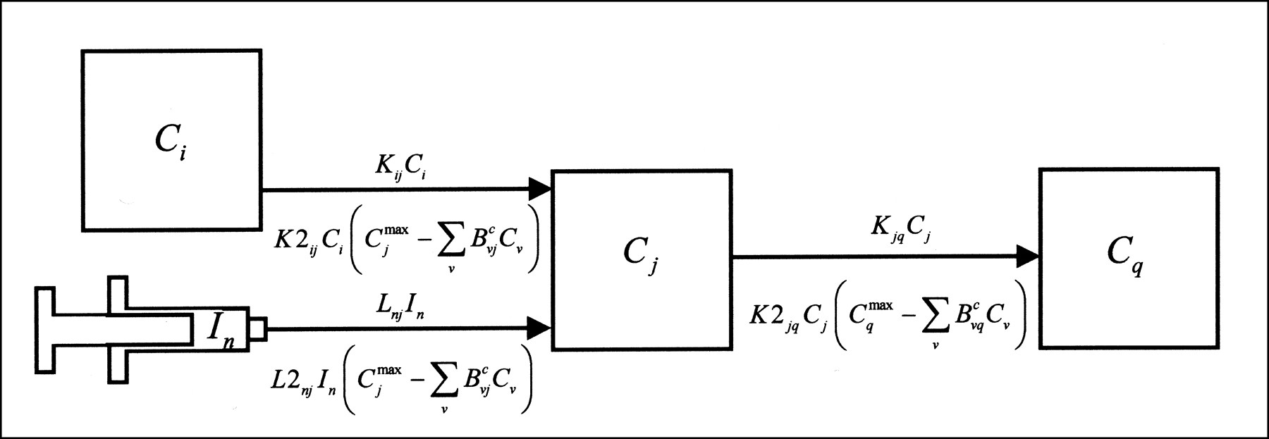
The mathematic framework for COMKAT is based on a building block approach for compartment models, which is shown in Figure 1. In the figure, Cj denotes the concentration in compartment j, and In denotes the concentration of input n. Compartment j may exchange with zero or more other compartments and zero or more inputs. As an example, one might consider the FDG PET model to be composed of two such building blocks, with Cj from one unit corresponding to FDG in the tissue and Cj from the other unit corresponding to FDG-6-PO4 in the tissue.

Building blocks used to define compartment models. Compartments are shown as rectangles. Arrows indicate unimolecular (labeled above arrow) and bimolecular (labeled below arrow) fluxes.
Compartment j is formally the recipient of fluxes from zero or more compartments i and zero or more inputs n, and it is the source of fluxes into zero or more compartments q. Each such flux is considered either unimolecular or bimolecular. For a unimolecular flux, the rate is dependent on the concentration in the source compartment or input. More specifically, the flux equals the unimolecular rate constant multiplied by the concentration of the source compartment or input. In contrast, in a bimolecular flux, the rate is dependent on both the concentration of the source compartment or input and the concentration of the receiving compartment. The flux equals the bimolecular rate constant multiplied by the concentration of the driving compartment or input and the concentration of open binding sites in the receiving compartment. This relationship is calculated as (Cqmax − Cq), where Cqmax is the total concentration of binding sites and Cq is the concentration of occupied sites. Note that Cqmax is the value at which Cq saturates, because the flux approaches zero as Cq approaches Cqmax. In some cases, more than one compartment corresponds to a single saturable pool of binding sites. Such is the case when the model includes multiple parallel sets of compartments to account for multiple injections of material, each with possibly a different specific activity (7–9). Thus, we generalize the calculation of available binding sites to (Cqmax − ∑v BvqcCv), where Bvqc is the coupling coefficient. Bvqc equals unity if compartments v and q correspond to a common pool of binding sites and equals zero otherwise.
In agreement with this framework, the equation describing the pharmacokinetics of compartment j is
 Eq. 1
Eq. 1


 where Kij is the unimolecular rate constant from compartment i to j, K2ij is the bimolecular rate constant from compartment i to j, Lij is the unimolecular rate constant from input i to compartment j, and L2ij is the bimolecular rate constant from input i to compartment j. Note that for a given compartment j, one expects physiologic uptake to be either nonsaturable or saturable. In the former case, K2ij will equal zero for all i. In the latter case, Kij will equal zero for all i. Analogous expectations hold for L and L2.
Output Equation.
The output equation relates compartment and input concentrations to the measurable quantities. The output equation appropriate for the majority of nuclear medicine data is
 Eq. 2
where Ml is output l of the model, Wul is the relative contribution of compartment u to output l, Au is the exponentially decaying specific activity of material in compartment u, and Xul is the relative contribution of input i to output l. The indicated integration accounts for the temporal averaging inherent to experimental measurements. The equation relates C and I, concentrations at specific points in time, to these values averaged over the time interval of a scan that begins at tb and ends at te. In the simple case, values of Wul might be set to one for compartments contributing to output l and zero otherwise. Alternatively, other values could be used to account for partial volume, scatter, or other effects. Analogously, Xul could be set to a value reflecting the contribution of intravascular radioactivity to the measurement.
Eq. 2
where Ml is output l of the model, Wul is the relative contribution of compartment u to output l, Au is the exponentially decaying specific activity of material in compartment u, and Xul is the relative contribution of input i to output l. The indicated integration accounts for the temporal averaging inherent to experimental measurements. The equation relates C and I, concentrations at specific points in time, to these values averaged over the time interval of a scan that begins at tb and ends at te. In the simple case, values of Wul might be set to one for compartments contributing to output l and zero otherwise. Alternatively, other values could be used to account for partial volume, scatter, or other effects. Analogously, Xul could be set to a value reflecting the contribution of intravascular radioactivity to the measurement.
To facilitate computation of Ml, we define and integrate the next equation along with the state (Eq. 1):
 Eq. 3
so that Ml may be calculated as
Eq. 3
so that Ml may be calculated as
 Eq. 4
Eq. 4
Example.
For the sake of concreteness, we digress briefly with an example of how the general form of the state and output equations may be used in a PET receptor model wherein there is a single output corresponding to the concentration of radioactivity in a region of interest. First, one defines compartment concentrations in terms of molar concentrations, because this is what drives ligand–receptor interactions. Second, one defines separate inputs I for the plasma concentration of ligand and for the blood concentration of radioactivity. The former is the source of radioactivity to the compartments, whereas the latter is used to account for vascular radioactivity by setting the appropriate Xul equal to the tissue vascular space. Third, values for Wul corresponding to free and bound compartments are set to equal the tissue extravascular space and thus define the contributions to the output. Finally, Au, the specific activity, is used to convert the molar concentration in compartment u to the measured quantity, which is radioactivity concentration.
Sensitivity Equations.
Often one uses the model output to fit experimental data to estimate values of model parameters that have physiologic significance. Typically, the parameter estimates are obtained by minimizing a weighted least-squares objective function
 Eq. 5
where P is the experimental data, ςli2 is (an estimate of) the variance of Pl(ti, ti+1), and θ is the vector of model parameters. To minimize φ, it is advantageous to use the output sensitivities—the derivatives of M with respect to elements of θ. To derive the appropriate expressions, we differentiate analytically the output equation
Eq. 5
where P is the experimental data, ςli2 is (an estimate of) the variance of Pl(ti, ti+1), and θ is the vector of model parameters. To minimize φ, it is advantageous to use the output sensitivities—the derivatives of M with respect to elements of θ. To derive the appropriate expressions, we differentiate analytically the output equation
 Eq. 6
Eq. 6
To evaluate dOl/dθj we differentiate analytically (Eq. 3) with respect to parameter θj and then change the order of differentiation (10) to obtain
 Eq. 7
which is an ordinary differential equation (ODE) that can be solved simultaneously with Equations 1 and 2 to obtain dOl/dθj . To evaluate Equation 7, the indicated derivatives on the right hand side are evaluated analytically as follows:
Eq. 7
which is an ordinary differential equation (ODE) that can be solved simultaneously with Equations 1 and 2 to obtain dOl/dθj . To evaluate Equation 7, the indicated derivatives on the right hand side are evaluated analytically as follows:
 Eq. 8
Eq. 8

 Eq. 9
Eq. 9
With the exception of dCu/dθj, the derivatives on the right hand sides of Equations 8 and 9 are evaluated analytically. For example, if Wul is vascular fraction, dWul/dθj equals unity when element j of the parameter vector θ is vascular fraction and equals zero if Wul is independent of θj. To evaluate dCu/dθj analytically, the state equation (Eq. 1) is differentiated, and the order of differentiation is changed to obtain
 Eq. 10


This too is an ODE that can be integrated simultaneously with the other equations to obtain dCu/dθj. To evaluate the right hand side of Equation 10, we proceed analytically with the differentiation to yield expressions of the form dCn/dθj, dCnmax/dθj, dKin/dθj, dK2in/dθj, dLin/dθj, and dL2in/dθj. Terms of the first type are solutions of the ODEs being solved, and the other terms have trivial values. For example, dKin/dθj equals unity if parameter θj is Kin and zero if Kin is independent of θj.
Jacobian Equation.
An ODE solver is used to solve numerically the state, output, and sensitivity equations, which are in the form
 Eq. 11
F is the vector-valued function defined according to Equations 1 through 10, and y is a vector of values of state, output, and sensitivity functions. To solve these equations, we used the stiff ODE solvers written by Shampine and Reichelt (11) that are distributed with MATLAB. As is common for stiff ODE solvers, these require use of the Jacobian J = dF/dy, which can be estimated by numeric differentiation or by differentiating F analytically. We chose the analytic route, because, among other things, it is more computationally efficient. These equations are omitted here for the sake of brevity but are included in the COMKAT System User Manual.
Implementation
COMKAT was developed within MATLAB 5.0 and consists of functions for defining compartment models, solving them to obtain model output, and estimating parameter values. These features are supported both by command line and graphic user interfaces. All functions were written as m-files, which maximizes portability, because they will run, without compilation or modification, on any computer with MATLAB 5.0 or newer.
RESULTS
Examples
Blood Flow.
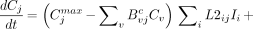
Figure 2 depicts a screen snapshot for the PET blood flow model (12–14). It contains one tissue compartment corresponding to an extravascular concentration of the tracer. It also contains two inputs—one corresponding to the molar concentration of the tracer and one corresponding to the blood radioactivity concentration of the tracer. This latter input is used to account for vascular radioactivity. While this model is sufficiently simple that vascular radioactivity could be modeled without separate inputs, we chose this representation to illustrate the approach that is necessary in more complex models.
Graphic user interface to define the blood flow model. Model was implemented by dragging compartments and inputs from left (labeled I3 and C3), switching to “Build Links” mode, and dragging arrows between inputs and compartments. For blood flow model, output includes contributions from Ct but not from “Junk,” which serves as a sink.
FDG Metabolism.
Figure 3 depicts a screen snapshot for the FDG metabolism model (15–19). It contains two tissue compartments corresponding to FDG and to FDG-6-PO4. Inputs were defined for both the plasma molar concentration of FDG and for the blood concentration of radioactivity. This latter input is used to account for vascular radioactivity.

Graphic user interface used to define FDG metabolism model. Implementation is analogous to that of blood flow model in Figure 2.
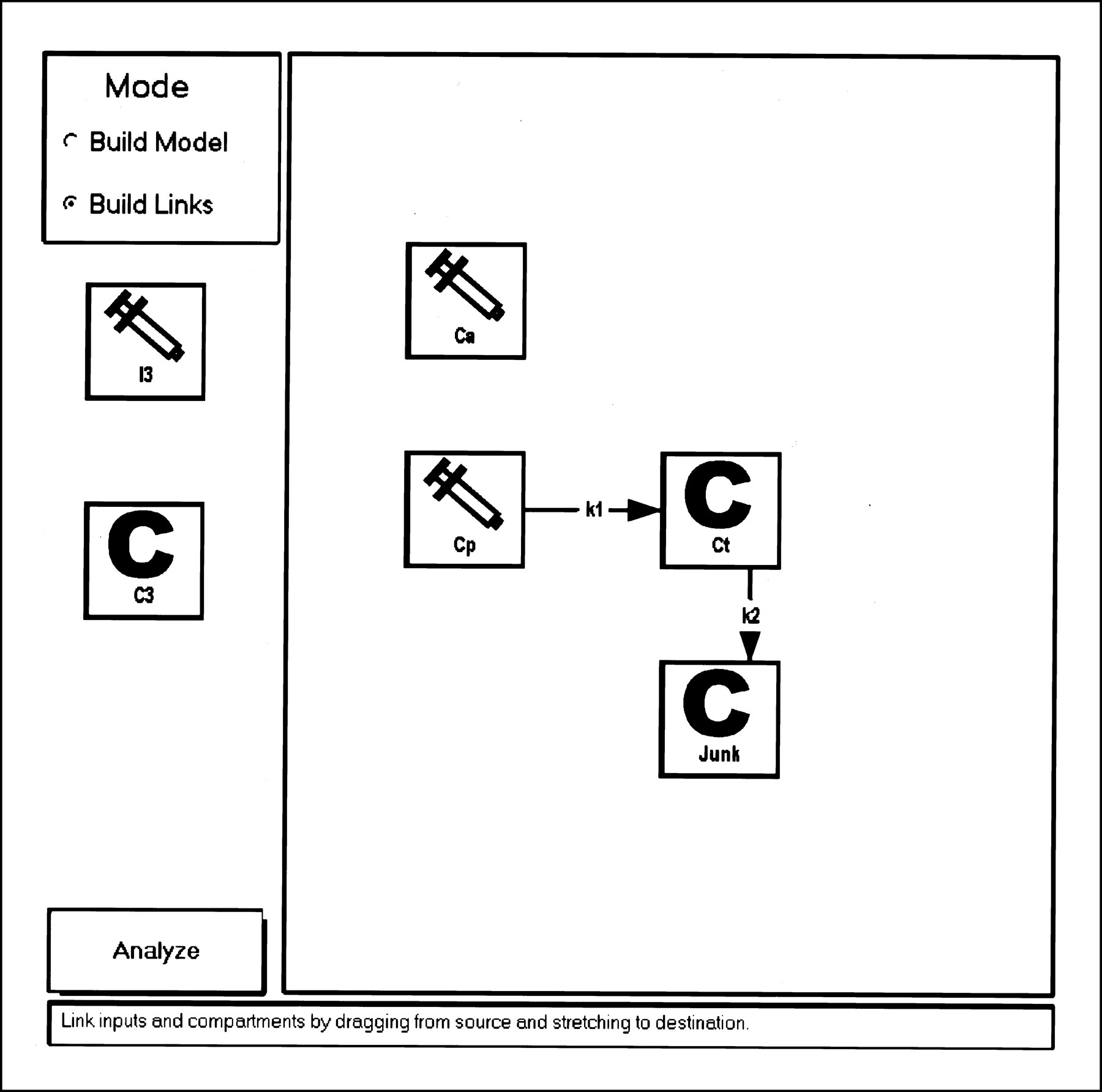
Receptor Model.
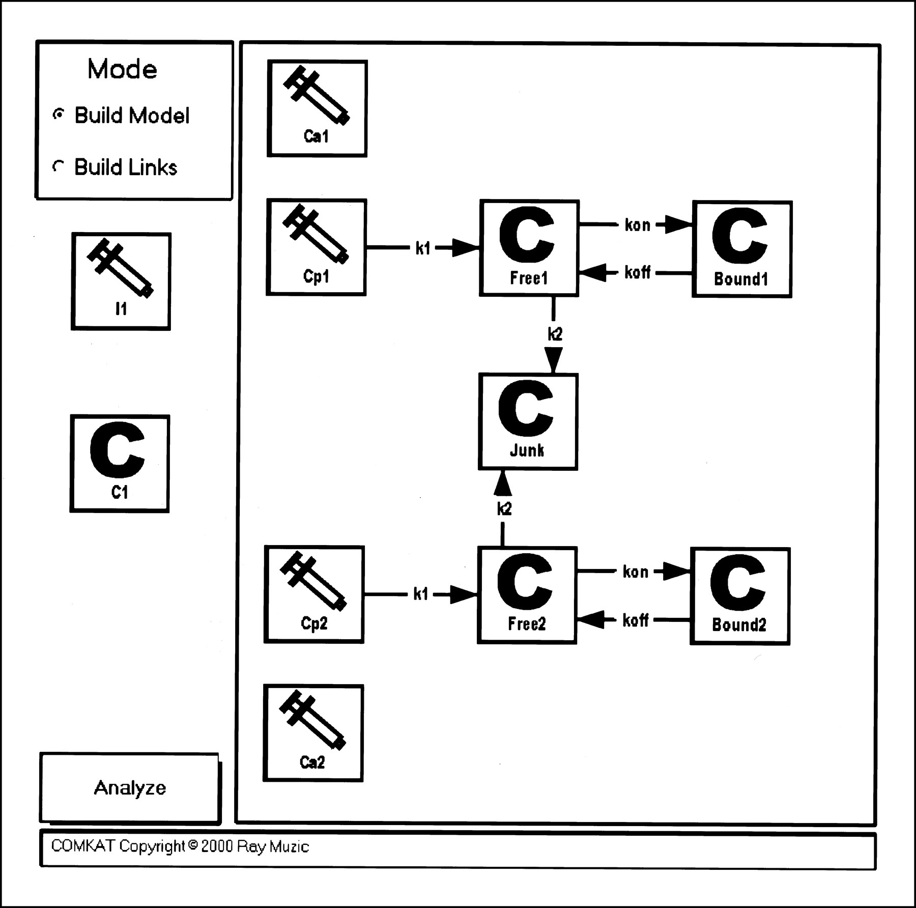
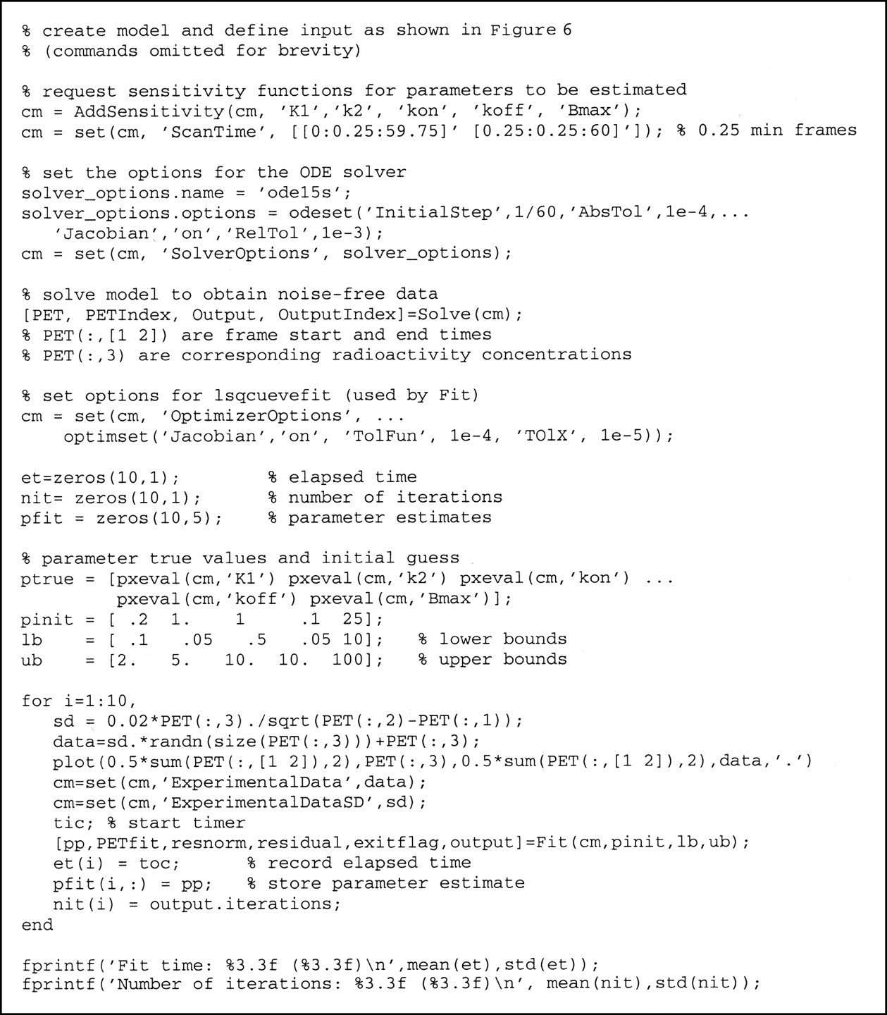
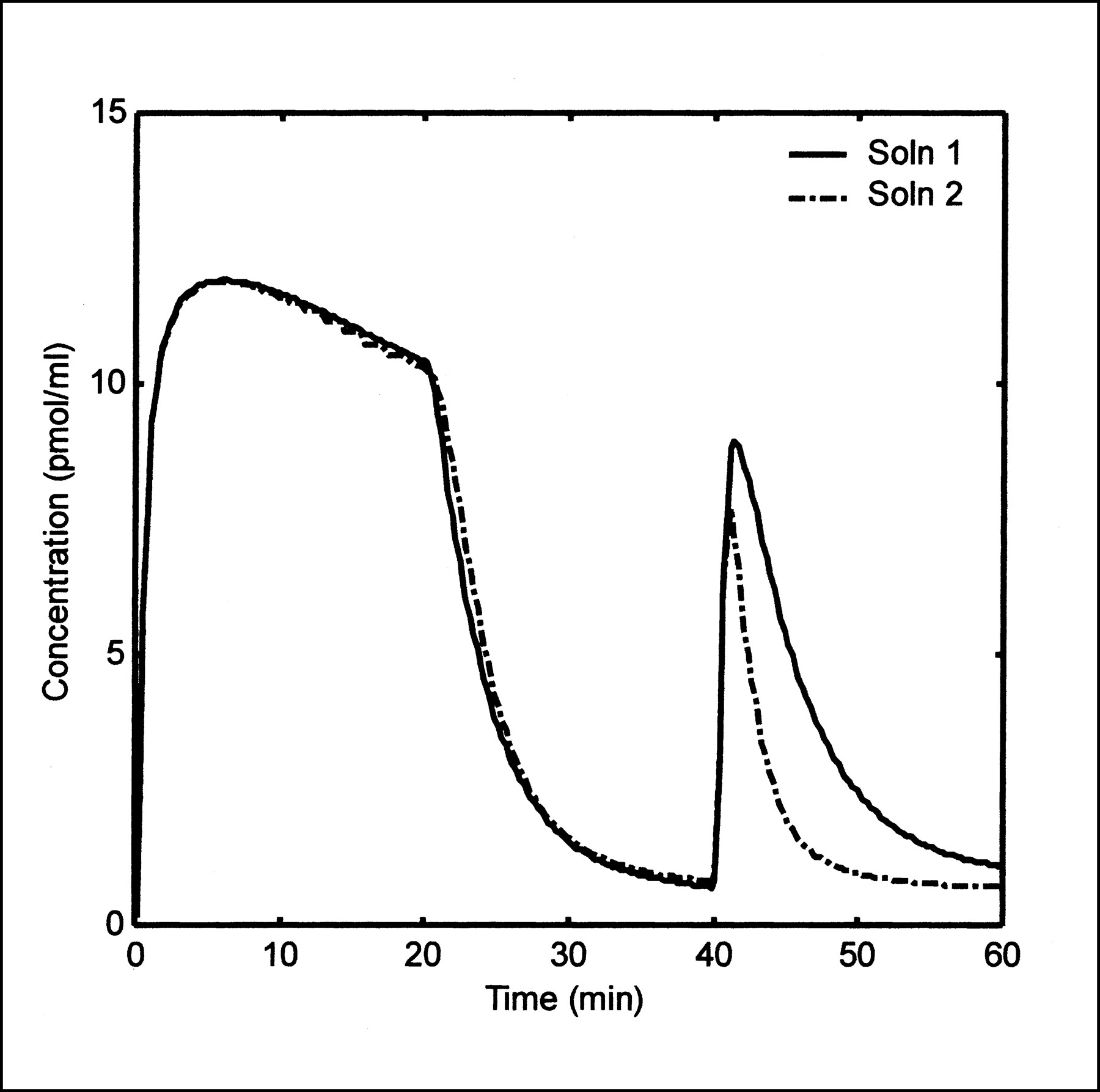
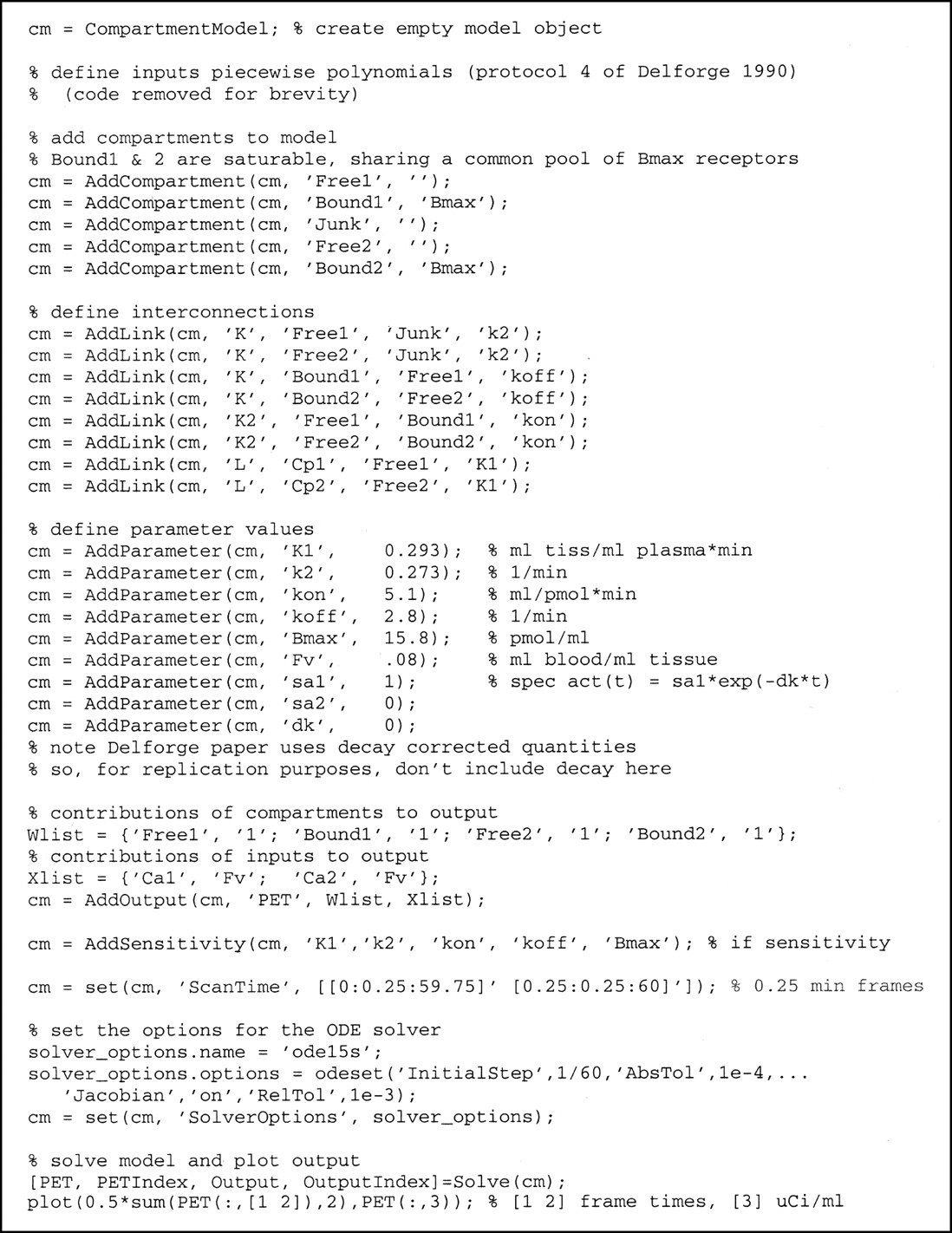
Figure 4 depicts a screen snapshot for the receptor model of Delforge et al. (7,8) which properly accounts for multiple injections of ligand at different specific activities (9). Example solutions are shown in Figure 5, and a MATLAB script showing command-line interface is included in Figure 6. For these solutions, model parameters were set to values defined as “solution 1” and “solution 2” (8), and the inputs were defined using data kindly provided by Jacques Delforge. The model output in Figure 5 agrees well with that shown elsewhere (Fig. 7) (7). Note that to reproduce this result, the contribution of vascular radioactivity to model output X was set to zero, and the model output was expressed in a molar concentration by setting initial specific activity to unity and the decay constant (ln 2/half-life) to zero.
Graphic user interface used to define receptor model. Implementation is analogous to that of blood flow model in Figure 2, except that saturation values are defined for “Bound1” and “Bound2” compartments using model parameter Bmax. Because same parameter was referenced as saturation value of both compartments, COMKAT treats this as indication of common pool of receptors.


Example plot from parameter estimation. Plot shows simulation data including “noise” (triangles), initial guess (dashed curve), and final fit (solid curve).
Validation
Model outputs for the three example models were validated by comparison with prior model-specific implementations of receptor models developed previously by us (20,21), by comparison with model solutions published by other institutions (8,9) and with analytic solutions of blood flow and FDG models.
Performance
Solving Model Equations.
Although COMKAT is written to solve compartment models of arbitrary, user-specified configurations, it is nevertheless efficient. This is illustrated in Table 1, which lists time to solve the three example models both with and without sensitivity functions, on a Pentium 2/366 (Intel Corp., Santa Clara, CA) notebook computer running MATLAB 5.3 and Windows NT 4 (SP4). Times were measured with MATLAB’s clock function, and the set of ODEs was solved with ODE15s (11), using absolute and relative tolerances of 10−4 and 10−3, respectively.
Computational Performance Summary
Parameter Estimation.
To evaluate COMKAT’s performance in parameter estimation, we created simulation data using the blood flow, FDG, and receptor models. Using the same input functions used for Solving Model Equations, simulated noise-free data were generated by solving the model using the “True” parameter values listed in Table 2 to obtain the outputs M1(ti,ti+1). Noisy simulation data were created by adding to the noise-free data a sample from a normal distribution with zero mean and 0.02M1(ti, ti+1)/ti+1 − ti SD. Using the weighted least-squares objective function (Eq. 5) with ς1i set equal to this SD, the parameter values were estimated from the noisy simulation data beginning with initial guesses listed in Table 2. In this process COMKAT’s “Fit( )” function made use of MATLAB’s “lsqcurvefit” (24) function to minimize φ(θ) with the lower and upper bound constraints listed in Table 2. For the FDG and receptor models, termination criteria for the minimization were set to 10−4 for TolFun and 10−6 for TolX. For the blood flow model, the same value for TolX was used, whereas the value for TolFun was reduced to 10−5 because of the relatively fewer data points in its simulated data.
Parameter Estimation Results
As an example, Figure 7 shows the noisy simulation dataset, the initial guess, and the fit from the receptor model. For all three models, 10 runs with independent noise realizations were performed. The mean (SD) of time required to estimate the parameters was 0.09 (0.03), 0.86 (0.16), and 12 (1.0) min for the blood flow, FDG, and receptor models, respectively. In all cases, the fits converged, and the parameter estimates were not significantly different from their true values (paired t test) in spite of a relatively poor initial guess. The MATLAB commands to perform this parameter estimation for the receptor model are given in Figure 8. The parameter estimation example shows robustness.
DISCUSSION
A key point regarding the model formulation and implementation is that arbitrary model configurations are supported. By this we mean that a user is not restricted to using predefined models distributed with COMKAT. Rather, any model of the user’s design can be set up. Moreover, COMKAT can support models with a large number of compartments. For example, we have already implemented models with 12 compartments. Thus, COMKAT might be useful beyond nuclear medicine in applications such as drug development, in which whole-body distribution models are used.
Several features of the model formulation are noteworthy. First, it is based on molar concentrations for the compartments because this quantity and not radioactivity governs the pharmacokinetics. Second, the model directly accounts for radioactive decay through the use of the time-varying specific activity Au. This approach is preferable to the alternative of precorrecting data for radioactive decay because this method facilitates use of optimal statistical weights in parameter estimation (25). Moreover, our approach of accounting for decay in the output equation can be shown analytically to produce model output identical to that obtained when radioactive decay is included directly in the state equations. Notably, our approach avoids the added complexity of including decay terms in the state equations. Third, the formulation supports multiple-injection receptor models in that both saturation and injections with different specific activities are addressed. Fourth, analytically derived sensitivity and Jacobian equations are used. This improves the numeric accuracy and computational efficiency compared with approximating these by numeric differentiation (10). It is important that, because we derived the sensitivity and Jacobian equations for the general case, no derivation is required on the part of the software user. Fifth, the formulation supports multiple output equations. This feature could be used, for example, to analyze data simultaneously from multiple regions, wherein some of the rate constants for some of the regions might be required to have a common value.
The examples illustrate that models of a range of complexities can be solved. Although we placed particular emphasis on the Delforge receptor model, because it is one of the more complex models, it is important to emphasize that the user is not constrained to use the models provided. Using the graphic user interface and without any mathematic derivations, a user can implement any model configuration he or she defines by simply positioning rectangles for the compartments and inputs and arrows for the connections. Alternatively, models may be implemented and solved from the command line (Figs. 6 and 8). This is particularly useful for automating data analysis tasks such as parameter estimation.
Figures 7 and 8 list the commands used in evaluating performance in solving model equations and in parameter estimation. A few points become apparent from these listings. First, no derivations were required on the part of the user. Second, an object-oriented syntax is used to define and solve models and to estimate parameters. This provides a simple syntax that is easily extendable while minimizing backward-compatibility problems.
One might expect that the computational performance would be poor because MATLAB is an interpreted language. The timing results show that this is not the case. Indeed, in implementing Equations 1 through 10, care was taken to avoid loops and to instead use MATLAB’s highly optimized matrix-vector operations to implement the summations.
In our timing results, we used ode15s to solve the system of differential equations. This solver is intended for solving stiff systems. One method for ascertaining whether a stiff solver is necessary is to simply compare solution times of a stiff solver and a nonstiff solver while keeping all other factors unchanged. The presence of stiffness can be diagnosed if the stiff solver solves the equations more efficiently. Indeed, this is the recommended approach for detecting stiffness in the MATLAB ODE Suite documentation (11). Applying this technique, we ascertained that the blood flow, FDG, and receptor models are stiff. Notably, because the ODE solvers in the ODE Suite use the same call syntax, switching between stiff and nonstiff solvers is nearly trivial; it requires only changing the name of the solver to call.
Other software for compartment modeling includes BLD (2), KMZ/PKIN (3), and SAAM/SAAM II (4), to name a few. In comparison with each of these, COMKAT has a unique combination of features that makes it particularly well suited for research. COMKAT supports saturable and nonsaturable kinetics, has analytic sensitivity equations, and can be run on any computer for which MATLAB is available. Moreover, users may integrate their own application-specific pre- and postprocessing tasks (e.g., input function smoothing, statistical summary) with COMKAT’s modeling analysis by implementing such tasks in MATLAB. Finally, MATLAB is distributed in source-code form without cost to interested researchers.
CONCLUSION
COMKAT is a MATLAB-based compartment- modeling package. We believe it has many features desirable for analysis of nuclear medicine data, and we use it routinely in our own research. COMKAT is available at www.nuclear.uhrad.com/comkat. We hope others find it useful and share improvements and new features.
Acknowledgments
The authors thank Daniel Pendergast, Joan Zhang, and Jigar Patel for contributions to the programming effort; Evan D. Morris for constructive comments made on a preliminary draft of the manuscript; Nathaniel Alpert for valuable discussions and for providing feedback on the software; and Larry Shampine for discussions on numerically solving sets of differential equations. This study was supported in part by National Institutes of Health grant R01 HL62399.
Footnotes
Received Aug. 9, 2000; revision accepted Dec. 12, 2000.
For correspondence or reprints contact: Raymond F. Muzic, Jr., PhD, Nuclear Medicine, University Hospitals of Cleveland, 11100 Euclid Ave., Cleveland, OH 44106.
REFERENCES
In this issue


Jump to section
Related Articles
Cited By...
- Spectral Clustering Predicts Tumor Tissue Heterogeneity Using Dynamic 18F-FDG PET: A Complement to the Standard Compartmental Modeling Approach
- Dopamine in the medial amygdala network mediates human bonding
- PET Imaging of {alpha}4{beta}2* Nicotinic Acetylcholine Receptors: Quantitative Analysis of 18F-Nifene Kinetics in the Nonhuman Primate
- Quantitative, Preclinical PET of Translocator Protein Expression in Glioma Using 18F-N-Fluoroacetyl-N-(2,5-Dimethoxybenzyl)-2-Phenoxyaniline
- Integrated Software Environment Based on COMKAT for Analyzing Tracer Pharmacokinetics with Molecular Imaging
- Uptake of 18F-Labeled 6-Fluoro-6-Deoxy-D-Glucose by Skeletal Muscle Is Responsive to Insulin Stimulation
- Spillover and Partial-Volume Correction for Image-Derived Input Functions for Small-Animal 18F-FDG PET Studies
- Arterial Input Function Measurement Without Blood Sampling Using a {beta}-Microprobe in Rats
- Change in Binding Potential as a Quantitative Index of Neurotransmitter Release Is Highly Sensitive to Relative Timing and Kinetics of the Tracer and the Endogenous Ligand