


Abstract
Tumor detection depends on the contrast between tumor activity and background activity and on the image noise in these 2 regions. The lower the image noise, the easier the tumor detection. Tumor activity contrast is determined by physiology. Noise, however, is affected by many factors, including the choice of reconstruction algorithm. Previous simulation and phantom measurements indicated that the ordered-subset expectation maximization (OSEM) algorithm may produce less noisy images than does the usual filtered backprojection (FBP) method, at equivalent resolution. To see if this prediction would hold in actual clinical situations, we quantified noise in clinical images reconstructed with both OSEM and FBP. Methods: Three patients (2 with colon cancer, 1 with breast cancer) were imaged with FDG PET using a “gated replicate” technique that permitted accurate measurement of noise at each pixel. Each static image was acquired as a gated image sequence, using a pulse generator with a 1-s period, yielding 40 replicate images over the 10- to 15-min imaging time. The images were or were not precorrected for attenuation and were reconstructed with both FBP and OSEM at comparable resolution. From these data, images of pixel mean, SD, and signal-to-noise ratio (S/N) could be produced, reflecting only noise caused by the statistical fluctuations in the emission process. Results: Noise did not vary greatly over each FBP image, even when image intensity varied greatly from one region to the next, causing S/N to be worse in low-activity regions than in high-activity regions. In contrast, OSEM had high noise in hot regions and low noise in cold regions. OSEM had a much better S/N than did FBP in cold regions of the image, such as the lungs (in the attenuation-corrected images), where improvements in S/N averaged 160%. Improvements with OSEM were less dramatic in hotter areas such as the liver (averaging 25% improvement in the attenuation-corrected images). In very hot tumors, FBP actually produced higher S/Ns than did OSEM. Conclusion: We conclude that OSEM reconstruction can significantly reduce image noise, especially in relatively low-count regions. OSEM reconstruction failed to improve S/N in very hot tumors, in which S/N may already be adequate for tumor detection.
Imaging with FDG PET is a valuable technique for tumor detection (1). Many oncology PET studies require imaging at several levels of the body to produce a nearly whole-body PET scan. This requirement often necessitates shortening the emission acquisition and shortening (or in some cases eliminating) the transmission scans to keep the total imaging time from becoming prohibitively long. These reductions in emission and transmission imaging time result in images that appear noisier than they would otherwise, potentially reducing the reader’s ability to detect tumors. Some investigators have noticed that reconstruction with iterative algorithms (e.g., the ordered-subset expectation maximization [OSEM] algorithm) produces images that seem visually less noisy than the equivalent images reconstructed with the standard filtered backprojection (FBP) algorithm (2–5). Many institutions have therefore considered switching to these iterative algorithms.
FBP reconstructions have well-understood noise characteristics; in fact, one can easily compute the noise present in FBP images (6,7). Iterative algorithms such as OSEM (8,9), however, are nonlinear, and their noise properties are far more complex (10). Theoretic studies (11) and phantom studies (2) have shown that iterative reconstruction should achieve better noise characteristics than does FBP. In addition, when simulated lesions were inserted into brain images, improved lesion detection was reported with iterative, compared with FBP, reconstructions (12). However, because accurate measurement of noise from patient images is difficult, few, if any, quantitative analyses of OSEM-reconstructed image noise in real patient images have been performed (13). Justification for the clinical use of the OSEM algorithm for oncology rests, therefore, primarily on the perception that OSEM images “look” better than FBP images and on the above-mentioned theoretic and simulation studies. As promising as these may be, further quantitative analyses using actual patient data seem warranted. We report here the results obtained with an acquisition technique (7) that permits accurate measurement of noise in clinical images, independent of any noise in the transmission data (if used) or of true spatial variations in image intensity. We used this method to compare the noise in FBP-reconstructed clinical images with the noise in OSEM-reconstructed clinical images, both with and without attenuation correction (AC). Because image noise is an important component of tumor detection, these measurements provide further insight into how, and under what circumstances, iterative reconstruction might improve diagnoses in whole-body FDG PET oncology imaging.
MATERIALS AND METHODS
Measuring Noise in Clinical Images
The statistical properties of the pixel values within an image can be computed if one acquires many independent replicate images of the radioactivity distribution. For example, one could acquire 40 separate sinograms at each bed position. If these 40 sinograms were acquired sequentially (e.g., using a dynamic acquisition), any changes in activity or activity distribution occurring between the first and the 40th scan (typically 10–20 min) would cause the 40 measurements not to be true replicates of each other, introducing errors into the statistical analysis. To solve this problem, we acquired the data as a gated set of images, in a manner identical to a cardiac gated study but using a pulse generator, not an electrocardiograph, as the gate signal. The pulse generator rate was set to 1 pulse per second. Because of computer memory limitations, the 40 replicate images were acquired as 2 sets of 20 gated images each. The gating process guaranteed that all the gated images in a set sampled the identical activity level and distribution, apart from any activity changes that might have occurred over the 1-s interval between the beginning and end of a gate. Therefore, the only differences between the sinograms in a gated set were caused by emission counting statistics. Each replicate image was reconstructed with FBP and with OSEM, once with AC and once with no AC (NAC). The SD and mean value of each pixel could then be measured for each of the 4 combinations (FBP + AC, FBP + NAC, OSEM + AC, and OSEM + NAC) by averaging the SDs and mean values obtained from each of the 2 gated sets. From these values, an SD image (the intensity of each pixel being proportional to the SD at that pixel) and a mean/SD image (i.e., a signal-to-noise ratio [S/N] image) were created. Even though noise at a pixel depends on AC, the computed SD of each pixel did not include transmission noise, because the same transmission scan was used for all 40 replicates.
Data Acquisition and Processing
All datasets were acquired on an Advance PET scanner (General Electric Medical Systems, Milwaukee, WI) with 18 detector rings, yielding 35 slices at a 4.25-mm center-to-center slice separation (14). FDG whole-body studies were performed in 2-dimensional mode (septa in place). The acquisition time was 10–20 min per bed position, with 5 or 6 positions per patient. The scanner was coupled to a pulse generator with a 1-s period to generate 2 groups of 20 replicate measurements per slice (50 ms per gate), or 40 replicates in all. Each emission acquisition was immediately preceded or followed by an 8-min (ungated) transmission scan. The arms of the patients were outside the field of view. Transmission scans were low-pass filtered in the transverse plane (full width at half maximum [FWHM], 15 mm), the standard procedure in our institution, and corrected for emission contamination. Replicate acquisitions were obtained for 3 patients: 2 with colon cancer and 1 with breast cancer. Four representative slices, each containing 40 replicate sinograms, were selected from each patient for analysis. The total counts per replicate sinogram ranged from 7,000 to 10,000 before AC.
Each replicate was precorrected for random noise and was either preprocessed for AC or left attenuated. Scatter correction (14,15) was performed for AC datasets only. Random noise, scatter, and AC can induce negative values that are not compatible with the Poisson model used in OSEM. Negative projection values were clipped to zero before reconstruction. OSEM and FBP were applied to the same zero-clipped datasets to prevent potential bias. The sinogram bins were also grouped by pairs to a bin size of 4 mm instead of the originally acquired 2 mm. This step was found desirable because it increased the S/N in each of the short replicate images without introducing correlations in the projection data. Each replicate was reconstructed into a 128 × 128 image (pixel size, 4 mm) with FBP (ramp filtered) and OSEM (3 iterations, 21 subsets, roughly equivalent to 63 iterations of the regular expectation-maximization algorithm). We verified that the resolution obtained with this number of iterations matched the resolution obtained with FBP by analyzing anatomic features in the images (hot spots on AC and NAC images, skin on NAC images) and fitting profiles of those features to gaussian functions. Estimates of FWHM were equivalent for FBP and OSEM (average FWHM difference, 0 ± 1 mm) for 17 anatomic features with sizes ranging from 12 to 20 mm for both OSEM and FBP. All replicate images were subsequently filtered with a gaussian filter (FWHM, 8 mm) before computation of the mean and SD images of each set to increase the S/N of the short replicate images. SD images were further filtered (FWHM, 8 mm) to reduce the errors in SD estimates. S/N images were obtained by dividing the mean images by their respective SD images. Finally, we computed an image percentage improvement, in which the intensity of each pixel represented the percentage improvement resulting from use of one method (i.e., OSEM or FBP) rather than the other. Thus, we could compare the S/N for OSEM and FBP (either with or without AC) by:
 if OSEM was better than FBP or
 Eq. 1
if FBP was better than OSEM.
Eq. 1
if FBP was better than OSEM.
%IFBP vs. OSEM was, for each pixel, either the percentage improvement resulting from use of OSEM over FBP, if OSEM was better, or the percentage improvement resulting from use of FBP over OSEM, if FBP was better. An image was made of the percentage improvement to allow visual and quantitative assessment of where, and by how much, the S/N of one method exceeded that of the other.
Simulation
The noise measurements characterize the noise in a single replicate, not in the full acquisition (the sum of the 40 replicate gates). Mean and variance will scale linearly with the average total count level for FBP, because FBP involves linear processing. A simulation was performed to verify that S/N scaled appropriately with increasing total counts in the data when using OSEM, because OSEM is a nonlinear process. The reference image was of an anthropomorphic torso phantom. The distribution was segmented into 4 components: lungs, hot background, heart cavity, and heart wall. An activity level was assigned to each component (lungs = 3, hot background = 6, heart cavity = 2, heart wall = 10), and a sinogram was generated with the same acquisition parameters (e.g., matrix size and pixel size) as in the patient studies, leading to a total of 18,786 counts. From this sinogram, 40 replicate sinograms with Poisson noise were generated for 30 count levels ranging from 1,878.6 to 1,878,600 (average total number of counts per replicate sinogram). No effect other than Poisson statistics was simulated (i.e., attenuation, random noise, and scatter were ignored). All sinograms were reconstructed with OSEM (3 iterations, 21 subsets). The S/N was computed at each pixel. Those estimates were averaged over each component (e.g., lungs and heart wall), giving an estimate of the S/N for each component at each count level.
RESULTS
Figure 1 shows the reconstructed images of 4 representative slices, chosen to illustrate 4 important anatomic situations: lungs (column A), normal liver (column B), liver with tumor (column C), and breast (column D). Each image in Figure 1 was computed by averaging the reconstructed images of each of the 40 replicates. For the images in column C, liver and tumors were very similar on 3 contiguous slices. This similarity allowed an additional 3-slice averaging of sinograms (for this column only) before reconstructing the replicates to determine whether the relative performances of OSEM and FBP remained unchanged even though the count level for column C was 2–3 times higher than for columns A, B, and D. The first row and the second row were processed with FBP and OSEM, respectively, with correction for attenuation (row 1 shows FBP-AC, row 2 shows OSEM-AC). Because some institutions do not perform AC, the third and fourth rows allow comparison of the FBP and OSEM algorithms when NAC is applied (row 3, FBP-NAC; row 4, OSEM-NAC). FBP images contained many negative values that were set to zero for improved display (but were not set to zero for quantitative analyses). Each pair of FBP and OSEM images (e.g., rows 1 and 2) are displayed with the same intensity range. Therefore, a quantitatively correct visual comparison of FBP and OSEM can be made for each slice. The same scheme was used to allow visual comparison of FBP and OSEM for non–attenuation-corrected images in rows 3 and 4.
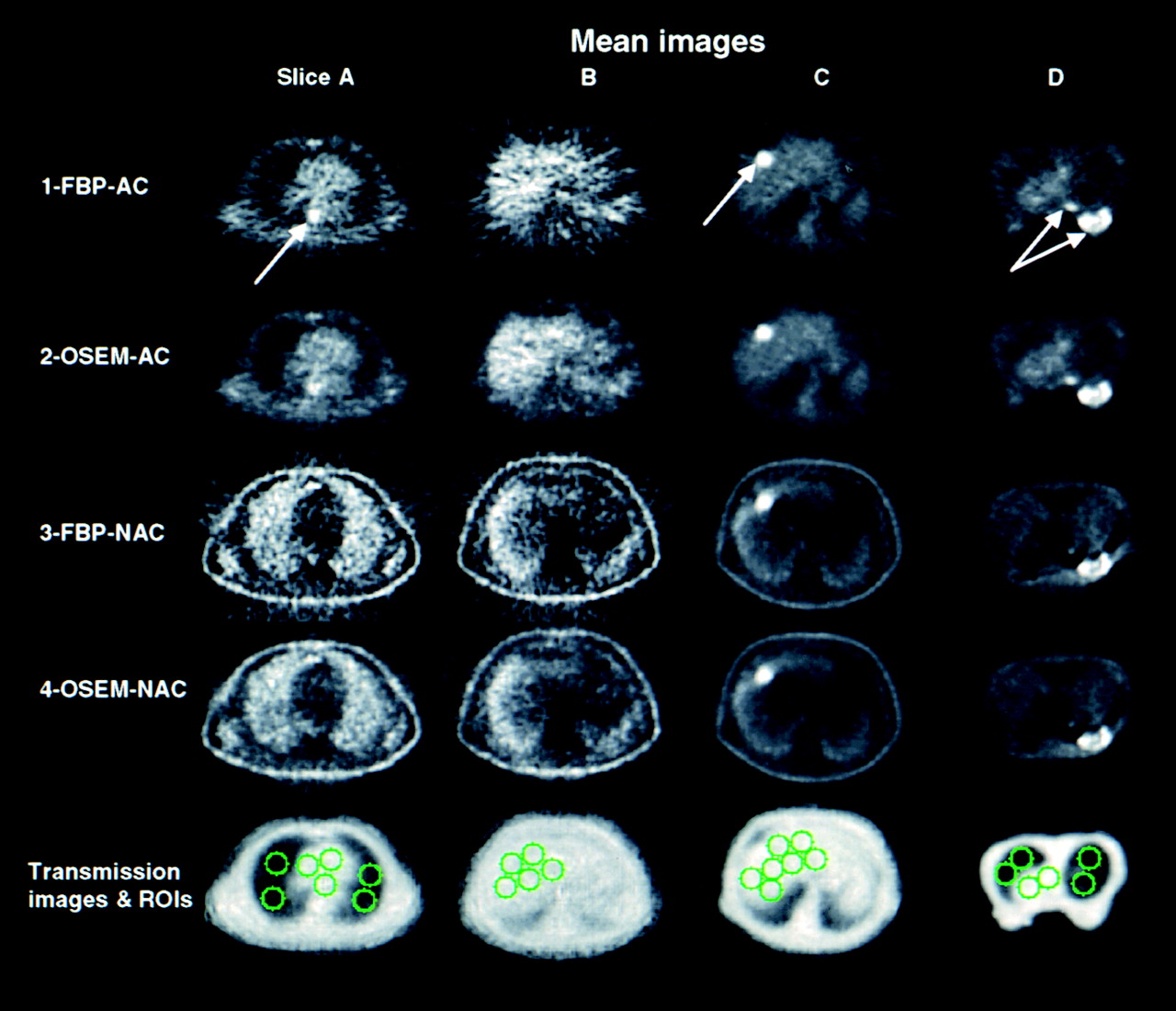
Mean of reconstructed image replicates for OSEM and FBP with and without AC for 4 different slices (A, B, C, and D). Negatives in FBP images are not displayed. For every slice, FBP-AC and OSEM-AC images are displayed to 1 common maximum, as are FBP-NAC and OSEM-NAC images. Hot tumor images have been clipped for display. Last row contains corresponding reconstructed attenuation maps with lung, heart, and liver regions of interest (ROIs). Whereas columns A, B, and C are displayed in standard supine position, breast images in column D are displayed in prone position.
The FBP images shown in row 1 of Figure 1 appear (by subjective visual assessment) to be noisier than the corresponding OSEM images in row 2, despite the fact that both images have the same resolution. Streaks, the hallmark of FBP reconstructions, are clearly seen in all slices of row 1 (FBP-AC), although most obviously for slices A and B. The OSEM-AC reconstructions (row 2) show no streaks. The periaortic region of high intensity in slice A, the liver tumor in slice C, and the breast and the mediastinal tumors in slice D are visible with both the OSEM and the FBP reconstructions (rows 1 and 2, labeled with arrows) despite the apparent increase in noise in the FBP-AC images. Apart from noise, the average measured activity distribution (and visual intensity pattern) of the images was nearly identical.
Percentage difference images ([OSEM − FBP]/OSEM) showed only an approximately random scatter of pixels, indicating no large differences in intensity between OSEM and FBP. Drawing regions of interest (ROIs) (all but 3 of which are shown on the corresponding attenuation images at the bottom of Fig. 1) and computing the average percentage difference between OSEM-AC and FBP-AC showed OSEM-AC to be lower by 1% ± 3% in the liver area (5 ROIs on slice B, 7 on slice C), by 3% ± 2% in bright tumors (1 ROI on slice C, 2 on slice D—ROIs are not shown but were drawn around the tumors labeled with arrows in row 1), and by 6% ± 3% in the heart. OSEM-AC was higher by 10% ± 10% in the lung (8 ROIs), possibly because of the constraint requiring OSEM pixels to remain positive.
Non–attenuation-corrected FBP and OSEM images are shown in rows 3 (FBP-NAC) and 4 (OSEM-NAC) of Figure 1. The images show the typical behavior caused by not performing AC: falsely high intensity in the lung and signal loss toward the center of the body (causing severe inhomogeneity in the liver slices). Because of this signal loss, the hot spot in the periaortic region of slice A, which is clearly seen in the attenuation-corrected images (rows 1 and 2) with both FBP and OSEM, is no longer visible in either the FBP or the OSEM images with NAC (rows 3 and 4). There is also (erroneously) high apparent uptake at the surface of the body, where total attenuation is low. Just as in the comparison of FBP and OSEM with AC (rows 1 and 2 of Fig. 1), the OSEM-NAC images appear to have less noise than the FBP-NAC images, although the degree of improvement is visually less dramatic. Again, the intensity distributions and magnitudes of the OSEM-NAC and the FBP-NAC images (apart from noise) were quite similar. One should remember that for NAC images, intensity values (i.e., the “signal” in NAC images) do not reflect the true activity distribution. Indeed, because both algorithms attempt to reconstruct an image from inconsistent projections, difference images showed some noticeable patterns, in particular at very low intensity regions of the image, where artifacts caused by lack of AC were most apparent. Nonetheless, the overall observed intensity was similar for the two, as can be seen in rows 3 and 4 of Figure 1. ROIs indicated OSEM to be only slightly greater than FBP in the liver (5% ± 14%) and to be slightly less in the lung (4% ± 5%). For the tumors, FBP exceeded OSEM by only 5% ± 2%. For the heart ROIs, FBP was less than OSEM by 36% ± 42% (because of the large attenuation at the heart, intensity was near zero, so small differences caused large percentage differences).
To quantify the noise differences between FBP and OSEM, we used the replicate images to compute SD maps. The brightness of each pixel in the SD map was directly proportional to the SD of that pixel value, as computed from the replicate data. Figure 2 shows the SD maps corresponding to the mean images of Figure 1, displayed in the same order. The first 2 rows of Figure 2 allow comparison of the image noise (as measured by the SD) for FBP (row 1) and OSEM (row 2) when AC is applied. Each SD map in row 2 is displayed with its maximum-value pixel given maximum brightness, and the identical display range was used for the corresponding map in row 1. Therefore, every pair of SD images (e.g., the pair of SD maps for slice A, rows 1 and 2, and the pair of SD maps for slice B, rows 1 and 2) is displayed on the same brightness scale and so can be directly compared visually. The SDs of the FBP images (row 1, Fig. 2) appear fairly uniform, showing little of the structure in the corresponding mean images (row 1, Fig. 1). In contrast, the SD maps of the OSEM images (row 2, Fig. 2) look similar to the corresponding mean images of Figure 1, except for the slightly reduced contrast. The noise at a pixel in the OSEM images seems strongly related to the intensity value of the corresponding pixel in the mean image. The SD values are high where the original image intensity (from Fig. 1) was high, and the SD is low where the original image intensity was low.
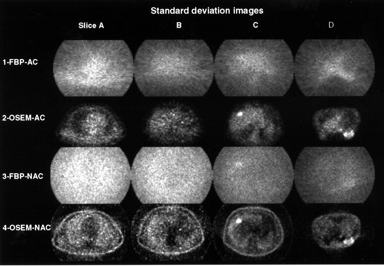
SD images displayed in same order as in Figure 1. Intensity of each pixel indicates magnitude of noise at that pixel. For every slice, FBP-AC and OSEM-AC images are displayed to 1 common maximum, as are FBP-NAC and OSEM-NAC images.
The SD maps for the NAC case are shown in rows 3 (FBP-NAC) and 4 (OSEM-NAC). Again, the level of noise in all regions of the FBP-NAC image is quite uniform and seems nearly unaffected by the local image intensity. In contrast, just as with AC, the OSEM-NAC SD map shows nearly the same structure as the original NAC image. Where the OSEM-NAC image is bright (e.g., the lungs), the noise is high, whereas where the image intensity is low (e.g., the center of the image), so too is the noise.
Figure 3 shows S/N images depicting the ratio of the signal intensity at each pixel to the noise at each pixel obtained by dividing the mean images of Figure 1 by the SD images of Figure 2. The S/N images of Figure 3 are all displayed on a single common gray scale (with S/N values > 2.2 set to maximum brightness) and are displayed in the same order as in Figures 1 and 2. Therefore, one can directly compare (visually) the S/N values between all the images of Figure 3. All S/N images had a similar range, despite the differences in AC and in the reconstruction algorithm. The S/N images for OSEM and FBP have a drastically different structure: FBP S/N images (rows 1 and 3 of Fig. 3) show a high S/N where the intensity is high and a low S/N where the intensity is low. OSEM S/N images (rows 2 and 4 of Fig. 3) are, on the other hand, much more uniform across the image.
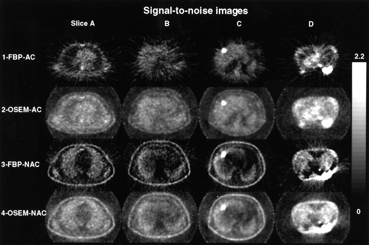
S/N images displayed in same order as in Figure 1. Intensity of each pixel reflects intensity of S/N at that pixel. Images are clipped so that all can be displayed on 1 common scale (0–2.2).
To make quantitative comparisons between the S/N levels in OSEM and FBP, we computed the percentage improvement images (as specified by Eq. 1), which are shown in Figure 4. In these images, the color scale allows one to visualize and quantify how much better or worse OSEM will be than FBP, in terms of S/N. Red and yellow indicate areas in which OSEM had a better S/N than did FBP, whereas blue and black indicate areas in which FBP had a better S/N. The amount of the difference is indicated by the color bar on the right. Improvements of greater than 100% were set to the maximum brightness (white for OSEM and black for FBP). In row 1, the attenuation-corrected FBP and OSEM algorithms are compared. In the areas of the lung (slices A and D), the images are bright yellow, indicating OSEM had far better (70% to >100% better) S/N in these regions. This finding was expected because the noise with FBP is nearly constant everywhere (Fig. 2) but the signal (Fig. 1) is low in the lung, whereas both signal and noise are low in the lungs with OSEM, giving a higher S/N than with FBP. In hotter regions (e.g., the liver in slices B and C and the heart in slices A and D), the images are a darker red, indicating a much smaller improvement of OSEM over FBP. In fact, the only areas of consistent blue are in the tumors themselves (slices C and D and, to a lesser extent, the periaortic hot spot in slice A). In these regions of localized high intensity, FBP actually gave a better S/N than did OSEM. However, these regions already had very high S/Ns for both methods.

S/N percentage improvement (%I) images. First row compares FBP-AC S/N images (Fig. 3, row 1) with OSEM-AC S/N images (Fig. 3, row 2). Second row compares FBP-NAC S/N images (Fig. 3, row 3) with OSEM-NAC S/N images (Fig. 3, row 4). Light blue background indicates that FBP and OSEM had comparable S/N. Red-to-yellow areas are where OSEM was better than FBP. Dark blue–to–black areas are where FBP was better than OSEM.
To quantify the S/N differences between FBP and OSEM, we analyzed the same ROIs described above (shown in the last row of Fig. 1): lungs (in slices A and D); liver, excluding tumors (in slices B and C); and tumors (in slices C and D). The average percentage improvement of OSEM over FBP was 160% ± 65% in the lung regions, 21% ± 9% in the liver regions, 29% ± 9% in the heart region, and −41% ± 7% in the tumor (the negative sign indicates that FBP was better there). Because the differences in mean values were small, the S/N changes were driven primarily by differences in noise between OSEM and FBP.
Row 2 of Figure 4 compares OSEM and FBP for the case when NAC is applied. In the lungs, only slight or near-zero improvement is seen using OSEM (dark red color). The more attenuated regions of the body (heart, mediastinum, and other soft tissue) had a much greater improvement with OSEM than with FBP. The exceptions are the tumors themselves, which again had a better S/N with FBP than with OSEM (dark blue colors). The same lung, liver, heart, and tumor regions as above were applied to the non–attenuation-corrected images, yielding an average percentage improvement for OSEM of 46% ± 13%, 84% ± 40%, 125% ± 49%, and −43% ± 7%, respectively.
Figure 5 shows the S/N plot with respect to the count level on a log–log scale for the simulated data. A regression over log(S/N) showed that the S/N was a linear function of the square root of the average count level (regression coefficient of 1.00 for all components of the simulated distribution). Therefore, the results of Figures 2–4 are expected to hold true even for count levels considerably above or below the 7,000–10,000 counts per replicate measured for the patients we studied.

(A) Emission distribution (segmented slice of anthropomorphic torso phantom study) used for simulating emission replicate sinograms at different count levels. (B) Plot of average S/N with respect to count level in reconstructed OSEM images in heart cavity, lungs, hot background (Bck), and heart wall of simulated distribution. Lines through data points are fits of data to straight line.
DISCUSSION
For some time, researchers have observed that iterative reconstruction methods, such as the OSEM algorithm, seem to produce less noisy images than does the conventional FBP method (2,10,11,13,16). Schiepers et al. (13) observed that in 18F-fluoride bone imaging of the pelvis and hips, in which the bladder was in the field of view, FBP produced images that were difficult to interpret clinically because of streak artifacts. Schiepers et al. found that OSEM appeared to eliminate these artifacts, resulting in images that they believed could be analyzed much more reliably (although for kinetic analysis, both FBP and OSEM gave similar parameters for 18F bone uptake). Theoretic studies and computer simulations (10,11,16) lend credence to these and other empiric observations of apparent reduction in noise by iterative reconstruction methods. Meikle et al. (2) compared S/Ns for FBP and OSEM in a mathematic phantom meant to represent the chest with inserted spheric tumors. Noise was simulated with a random, approximately Poisson, number generator. Compared with FBP, OSEM improved the S/N (defined slightly differently from our definition) from 68% to 168%, although this result depended on the number of iterations used for OSEM. In another study, simulated brain tumors were introduced into real brain images (12) and the ability of physicians to see the artificial tumors with OSEM and FBP reconstructions was compared. “Borderline” artificial tumors (i.e., tumors not differing much from background and therefore difficult to detect reliably with FBP images) were slightly easier to see with OSEM.
As mentioned previously, the linearity of the FBP process allows one to make theoretic predictions of the noise that will occur in a real, clinical FBP image. The nonlinearity of the OSEM algorithm makes such a computation exceedingly difficult (to our knowledge, it has never been achieved for clinical images) and is the reason that many previous investigations were based on simulations. Haynor and Woods (17) proposed an elegant “bootstrap/jackknife” method for creating a sort of “pseudo-replicate” dataset based on certain statistical assumptions, using list mode acquisitions. Using the gated replicate measurement method, we could make direct S/N measurements on actual clinical FDG PET scans without relying on any assumptions or simplifications that might be necessary in some simulations. These replicate measurements were then used to determine whether OSEM resulted in S/N improvement over the FBP method, and if so, in what parts of the image and by how much. Such a comparison is meaningful only if the resolution of the 2 reconstructions is matched. Resolution assessment is straightforward for FBP-reconstructed images but complex for OSEM images, because at the limited number of iterations used here and in clinical practice, resolution may differ for different objects within the image, depending on their relative size and intensity (18). By selecting several structures in the actual image data and inferring resolution from those structures, we believed we had objectively determined the number of iterations required, although the finite size of the objects used made such determinations difficult. Nonetheless, our choice of 63 effective iterations was slightly greater (and therefore more in favor of FBP in terms of noise) than that of Llacer et al. (11), who showed OSEM and FBP to match with a ramp filter after 35–45 iterations, and was similar to that of Meikle et al. (2), who optimized the number of iterations according to tumor size, with a minimum of 8 iterations and a maximum of 64 iterations. Certain unusual distributions of uptake for which the number of iterations used here may be insufficient are possible (19) and may introduce some bias. If more iterations are needed, the noise in the OSEM images will be higher. However, we believe that the situations studied here spanned a reasonably wide range of practically encountered clinical situations.
The data from Figure 1 showed that FBP and OSEM gave nearly identical signals, especially when AC was applied. That is, apart from noise differences, the mean intensity of the 2 image sets was very similar. Therefore, the S/N comparison reduces to a comparison of noise. Figure 2 shows the image noise for OSEM and FBP. FBP produces noise that is quite uniform throughout the image. The noise is almost completely uniform when NAC is applied but is still relatively uniform even with AC. This phenomenon had been predicted (6,20) from theoretic considerations. Most of the noise is caused by high-count projection lines. Even though high-count projection lines have a low percentage of noise, they have high absolute noise that, when backprojected across low-count areas (e.g., the lung), produces a high percentage of noise in the low-count regions. This is the reason that noise in the lung regions of FBP images is so high. The OSEM algorithm behaves differently. When a pixel value is high, the noise at that pixel is high, and when a pixel value is low, the noise is low. The noise from hot pixels does not spread out over other pixels, as with FBP. This is seen clearly in Figure 2, and this general behavior has been suggested by theoretic considerations (10,11). We expect OSEM, therefore, to most surpass FBP in regions of the image where counts are comparatively low. This is exactly what is observed in Figures 3 and 4: the lungs show the greatest improvement with OSEM in the attenuation-corrected images. In hotter areas, FBP and OSEM have a comparable S/N and there is less to be gained by using the OSEM method. In fact, in the very localized hot tumors examined in this study, FBP actually had a better S/N than did OSEM. These hot local tumors, however, already had such a high S/N that their detection might be less at issue. Interestingly, without AC, OSEM most surpasses FBP in the most attenuated areas, not in the lung. This finding is expected because, with NAC, the most attenuated areas have lower measured relative uptake.
The data of Figure 4 show that in most parts of the image, OSEM produces a better S/N than does FBP. This finding is true regardless of whether AC is performed. The improvement was greatest in the dimmer parts of images that contained both low-intensity and high-intensity regions and was smallest in the brighter parts of the images. In fact, FBP gave a better S/N at the site of the tumors themselves. Therefore, it is possible that OSEM would not improve detection of bright tumors embedded in a hot background (e.g., tumors in the liver). This possibility is consistent with our findings from the liver tumor of Figure 4 with AC. In those data, although S/N in the normal liver background tissue improved 21% with OSEM, S/N in the hot tumor was reduced 41%. The situation would be different for a less intense tumor, especially if it were in a lower intensity background region such as the lungs (with AC), where the improvements in S/N were found to be greater than 100%, and especially if the tumor had an intensity not much greater than background intensity. Such marginally detectable tumors would presumably be the most clinically interesting circumstance, and our data suggest that the S/N in such tumors would be significantly better with OSEM, making their detection easier with OSEM than with FBP. However, tumor detection depends on many other factors besides the S/N of the tumor—most notably on the relative signal and noise in both the tumor and its surrounding tissue.
The one situation not studied here was that of tumors near a hot bladder (as studied by Schiepers et al. (13)). The arguments above indicate that OSEM would produce a large percentage improvement over FBP in this situation (as supported by the data of Schiepers et al.).
One might think that the dataset used here to compare FBP and OSEM could be used equally well to quantitatively compare noise in attenuation-corrected and non–attenuation-corrected image sets. Unfortunately, comparisons of AC versus NAC are more difficult than comparisons of FBP versus OSEM. The “signal” itself is very different between AC and NAC images, as is the tumor-to-background contrast. In NAC images, the tumor-to-background contrast can also vary markedly from one side of the tumor to the other, because signal falls off so rapidly toward the center of the patient. The validity of using the S/N image for comparing AC and NAC images is made suspect by these difficulties, and for this reason, we did not attempt such comparisons.
Finally, the knowledge of each pixel’s variance does not describe the noise entirely. Noise texture was not considered, and it is possible that differences in noise texture exist between FBP and OSEM and that some observer retraining will be required to optimize visual interpretation of OSEM images.
CONCLUSION
We compared quantitative measures of noise in clinical PET images reconstructed with an iterative method (OSEM) and with the conventional FBP method. Forty replicate images were acquired for each patient and were reconstructed with each method. Over most regions of the images, OSEM resulted in better S/Ns than did FBP, regardless of whether AC was performed. The improvement was most dramatic in the cold regions of images, such as of the lungs (with AC), that had both cold and hot regions. In such cases, improvements averaged 160%. Improvements were less dramatic in hotter areas such as the liver (averaging 25% improvement in the AC images), and in very hot tumors FBP actually produced higher S/Ns than did OSEM. We judged that this last occurrence did not preclude the use of OSEM because these tumors were already easily detectable. The improved performance of OSEM resulted principally from the ability of the algorithm to localize noise, with hot areas having high noise and cold areas having low noise. In contrast, because FBP images produced noise that was more uniform over each image, high noise from hot areas spread out over large parts of the image and caused poor S/Ns in low-count regions. On the basis of our noise measurements, we believe that tumor detection may be better with OSEM than with FBP regardless of whether AC is used.
Footnotes
Received Nov. 27, 2000; revision accepted May 2, 2001.
For correspondence or reprints contact: Stephen L. Bacharach, PhD, Bldg. 10, Room 1C401, National Institutes of Health, Bethesda, MD 20892-1180.
REFERENCES
In this issue


Jump to section
Related Articles
Cited By...
- Assessment of Minimum 124I Activity Required in Uptake Measurements Before Radioiodine Therapy for Benign Thyroid Diseases
- The Effect of Misregistration Between CT-Attenuation and PET-Emission Images in 13N-Ammonia Myocardial PET/CT
- The effect of adaptive iterative dose reduction on image quality in 320-detector row CT coronary angiography
- Image quality of multiplanar reconstruction of pulmonary CT scans using adaptive statistical iterative reconstruction
- Optimization of the Injected Activity in Dynamic 3D PET: A Generalized Approach Using Patient-Specific NECs as Demonstrated by a Series of 15O-H2O Scans
- "Flying Through" and "Flying Around" a PET/CT Scan: Pilot Study and Development of 3D Integrated 18F-FDG PET/CT for Virtual Bronchoscopy and Colonoscopy
- Comparison of 2-Dimensional and 3-Dimensional Acquisition for 18F-FDG PET Oncology Studies Performed on an LSO-Based Scanner
- Influence of Reconstruction Iterations on 18F-FDG PET/CT Standardized Uptake Values
- Quantitative Comparison of Analytic and Iterative Reconstruction Methods in 2- and 3-Dimensional Dynamic Cardiac 18F-FDG PET
- Number of Iterations When Comparing MLEM/OSEM with FBP
- Clinical Implications of Different Image Reconstruction Parameters for Interpretation of Whole-Body PET Studies in Cancer Patients
- Postinjection Transmission Scanning in Myocardial 18F-FDG PET Studies Using Both Filtered Backprojection and Iterative Reconstruction
- PET Instrumentation and Reconstruction Algorithms in Whole-Body Applications