


Abstract
The magnitude of the injected activity (A0) has a direct impact on the statistical quality of PET images. This study aimed to develop a generalized method for maximizing the statistical quality of dynamic PET images by optimizing A0. Methods: Patient-specific noise-equivalent counts (PS-NECs) were used as a metric of the statistical quality of each time frame of a dynamic PET image. Previous methodology developed to extrapolate the NEC as a function of A0 was extended to dynamic PET, enabling the NEC to be extrapolated as a function of both A0 and the time after injection. This method allowed A0 to be optimized after a single scan (at a single A0), by maximizing the NEC within the time interval for which the parameter estimation is most sensitive. The extrapolation method was validated by a series of 15O-H2O scans of the body acquired in 3-dimensional mode. Each patient (n = 6) underwent between 3 and 6 scans at 1 bed position. The injected activities were varied over a wide range (140–840 MBq). Noise-equivalent counting rate (NECR) versus A0 curves and the optimal injected activities were calculated from each injection. Results: PS-NECR versus A0 curves as extrapolated from different injected activities were consistent (coefficient of variation, typically <5%). The optimal injected activities for an individual, as derived from these curves, were also consistent (maximum coefficient of variation, 4.3%). For abdominal (n = 4) and chest (n = 1) scans, we found optimal injected activities of 15O-H2O in the range of 220–350 MBq for estimating blood perfusion (F) and 660–1,070 MBq for estimating the volume of distribution (VT). Higher optimal injected activities were found in the case of a pelvic scan (n = 1; 570 MBq for F and 1,530 MBq for VT). Conclusion: PS-NECs are a valid and generic method for optimizing the injected activity in PET, allowing scanning protocols to be improved after the collection of an initial, single dynamic dataset. This generic method can be used to estimate the optimal injected activity, which is specific to the patient, tracer, PET scanner, and body region being scanned.
Significant levels of statistical noise in PET images are a common problem, especially when examining small structures or when data are acquired over a short period. The signal-to-noise ratio (SNR) of the PET images (SNRIMG) can be maximized through optimization of the scanning protocol. Optimization of the injected activity (A0) is of particular interest, because it has a direct impact on the image quality.
Noise-equivalent counts (NECs) are a measure of the statistical noise present in the projection data (1). NEC versus activity curves as measured in standard phantoms are commonly used to compare the performance of different PET scanners (2). NECs can also be useful for the optimization of the injected activity (3–6), scanner setup (7), and scanner design (8). By considering the statistical effects of correcting the data for unwanted random and scattered events, NECs provide a global estimate of the statistical quality of the remaining counts. The noise-equivalent counting rate (NECR) is the NEC per unit time and is given by: Eq. 1where T, S, and R are the average rates of true, scattered, and random coincidences, respectively, as acquired during the given time frame and evaluated within the boundaries of the object in projection space (1). k is assigned the value of 1 for a noiseless randoms correction and 2 for randoms correction via the direct subtraction of delayed coincidences. The formulation of the NEC is such that the SNR of the non-scattered true counts is the square root of the NEC collected. In the absence of scatter and randoms, the NEC is equal to the total true coincidences.
NEC methodology can be applied to patient data to optimize scanning protocols. The relative contributions of true, random, and scattered coincidences change with activity in a manner that is dependant on many factors: the distribution of activity within the subject, the region of the body being scanned, the amount and distribution of body mass, and the design and technical performance of the PET scanner. However, if the relationship between the NECR and A0 can be estimated for a given group of subjects, one has the opportunity to optimize A0 or the scan duration.
For filtered backprojection (FBP) image reconstruction, the maximization of NEC is expected to maximize SNRIMG for most regions within the body (9). On this basis, Watson et al. (3,10) developed a method to optimize A0 that is applicable to clinical 18F-FDG. At the heart of this methodology is the ability to extrapolate an NECR-A0 curve that is specific to an individual patient, using data acquired from that patient at a single injected activity. The validity of this method for an individual patient could not be fully assessed, because each subject in the study was scanned only once at a single injected activity.
This study meets 3 main aims. First, the patient-specific NECR (PS-NECR) method of Watson et al. (3,10) was extended to incorporate optimization of A0 for dynamic PET. This allowed PS-NECR-versus-time curves to be extrapolated for many possible injected activities. Second, the validity of the new method was qualified in a patient study, in which 6 cancer patients were each given between 3 and 6 injections of 15O-H2O at injected activities that varied in magnitude but were similar in all other regards. Such a validation is rarely performed because it requires multiple scans of the same subject over a range of injected activities, which is not practical with 18F- or 11C-labeled compounds. Finally, we estimated the injected activities that were optimal for measurements of perfusion (F) and the volume of distribution of water in tissue (VT), as derived from dynamic 15O-H2O scans of the body using a lutetium oxyorthosilicate (LSO)–based 3-dimensional (3D) PET/CT camera. A preliminary report of this work has been presented previously (11).
MATERIALS AND METHODS
Scanner Hardware
All scans were obtained on a Biograph-6 HiRez scanner (Siemens Molecular Imaging Inc.) (12). This is a whole-body, 3D PET/CT scanner with LSO crystals, fast (Pico 3D) electronics, and a short coincidence timing window (4.5 ns). Images were generated using the standard manufacturer's software. This includes simulation-based scatter correction and CT-derived attenuation correction. Randoms correction was performed via the direct subtraction of delayed coincidences. After Fourier rebinning of the 3D dataset, image reconstruction was performed for each image plane by a direct inverse Fourier transform of the rebinned projection data (similar to FBP). Although iterative reconstruction (ordered-subset expectation maximization [OSEM]) was also available for this scanner, it was not used in this study because of its additional uncertainties in absolute quantification (13,14).
Measurement of Scanner Live-Time Functions
All PET scanners are subject to appreciable counting losses when operating at high counting rates. This occurs as a result of detector and electronic dead-time; coincidences that would otherwise be recorded are lost. The live-time fraction characterizes this loss and can be defined as the fraction of counts that are recorded, compared with those recorded at a low counting rate. Live-time fractions are thus close to 1 at low counting rates and are less than 1 at high counting rates. The live-time fraction for a particular detector is often approximated by a function of the singles counting rate of the detector. This facilitates a correction for dead-time effects, preserving quantitation. To enable the extrapolation of patient counting rates (as in the study by Watson et al. (3)), a common live time is assumed for all detectors. We assumed that this live time, when calculated from the total singles counting rate, was independent of the object being scanned. Scanner live-time functions can then be measured in a phantom study and applied to patient data. In this study, singles were defined as detected photons that meet the energy discrimination (425–650 keV).
Whole scanner live-time functions for the Biograph were measured experimentally using the National Electrical Manufacturers Association NU 2 counting-rate phantom (2). This 20-cm-diameter, 70-cm-long solid polyethylene phantom was centered in the 16-cm axial field of view (FOV) of the scanner. The phantom has a small (6.4-mm diameter) hole along its axial extent, at a radial offset of 4.5 cm. A plastic tube was threaded through the phantom, into which a solution of 11C was injected. After a CT scan, PET list-mode data were acquired for 300 min (about 15 half-lives) and rebinned into 60 frames of 5 min. The initial activity was 943 MBq, of which approximately 20% was within the coincidence FOV. The decaying data were used to estimate the scanner live-time functions. As in the study by Watson et al. (3), the global counting rates for singles (s), non-scattered trues (T), and randoms (R), as collected in the absence of detector dead time, are related to the activity (a) in the object by: Eq. 2cs, cT, and cR are object-specific constants. sint represents the contribution of singles arising from the 176Lu background (15), for which aint is the equivalent radioactivity required to produce this counting rate (aint = sint/cs). In reality, each of these counting rates is reduced by a live-time factor. Incorporating these factors into Equation 2 we find:
 Eq. 3where fs, fT, and fR are the live-time functions for the singles, trues, and randoms counting rates, respectively, formulated as functions of s.
In the phantom experiment, the object-specific constants and sint were calculated from linear fits to the low-counting-rate data (s < 1.3 Mcps, a < 9 MBq, 17 frames), where Equation 2 is used (which assumes live-time fractions of 1). Equation 3 was then rearranged and used to calculate the live-time fractions for each frame, that is, over the entire range of counting rates: Eq. 4
Eq. 4
The 3 live-time functions were estimated as functions of the singles counting rate by fitting second- or third-order polynomials to these data. Scattered coincidences (S) can be incorporated into Equations 2–4 by assuming a counting rate–independent scatter fraction, allowing T(a) to be replaced by (T + S)(a). We chose this approach, modeling the scattered and non-scattered true coincidences jointly.
Extrapolation of PS-NECR-A0 Curves
Following the method of Watson et al. (3), the global counting rates for singles, randoms, and trues (including scatter) are extrapolated as a function of the injected activity for the specific individual, using measurements of these counting rates as obtained at a single activity. The method uses the phantom-derived live-time functions for trues, randoms, and singles counting rates.
From the measurements at a single A0, the object-specific constants (cT, cR, and cs) are determined (for each time frame) by rearrangement of Equation 3. Now including scattered coincidences, this yields: Eq. 5We assume no excretion of radioactivity from the subject, calculating a as a = A0e−λt, where t is the time since injection and λ is the decay constant of the radioisotope. Equation 3 can also be solved to find a, (T+S), and R as functions of the singles rate,
 Eq. 6
Eq. 6
These functions can be sampled at frequent intervals over a wide range of singles counting rates. Because a(s) is a monotonic function over the activities of interest, the extrapolated coincidence counting rates can be easily plotted against a or against A0 by including a decay correction. The scatter fraction (sf), defined as S/(T+S), is obtained from the scatter correction software of the scanner. The extrapolated counting rates, together with the scatter fraction, allows for the calculation of the NECR using Equation 1, with k assigned the value of 2 in this instance.
An estimate of the NECR is thus obtained over a wide range of injected activities, as extrapolated from measurements at a single activity. We term this an NECR-A0 curve for the specified time frame.
All coincidence rates (and the resulting scatter fraction) used to extrapolate the NECR-A0 curves are evaluated only over the portion of the sinogram containing the object. This is determined from the attenuation correction sinogram, using a threshold of 1.1. All the required data are reported by the scatter correction software (16). Because a randoms sinogram is not normally available on this system, the randoms sinogram is assumed to be uniform and calculated from the total randoms counting rate. This assumption has been shown to be valid in the case of clinical 18F-FDG (3).
Generation of NECR Time Curves
The NECR is dependent on both the distribution and the magnitude of radioactivity within an emitting object. After a bolus injection of 15O-H2O into a patient, significant changes in both the distribution and the magnitude of radioactivity occur with time. The latter is due to the radioactive decay of 15O (half-life, 2 min) during the course of the scan (6 min). The patient's NECR thus depends on both A0 and the time since injection. The dynamic PET scan cannot then be described by a point on a single NECR-A0 curve but is instead described by a time series of points on a time series of NECR-A0 curves. This time series is obtained by dividing the acquired patient data into short time frames and performing an NECR-A0 extrapolation on each frame individually. When combined, these NECR-A0 curves form an NECR–A0–time surface. Linear interpolation of this surface allows the NECR to be estimated as a function of time for any A0, providing that the singles rate remains within the range of the measured live-time functions. We term this an NECR time curve for the specified A0.
Validation of Methods with Patient Data
The counting rate extrapolation method was validated in a dose-ranging study, in which 6 cancer patients were each given a series of controlled injections of 15O-labeled water. We assume that the time course of the radioactivity distribution is the same for each injection but scaled in magnitude by A0. Requirements for this are minimal patient movement, no significant change in the patient state (e.g., heart rate), and a consistent method of tracer administration. The intravenous injections were controlled using an automated system (Radiowater Generator; Hidex Oy), in which each bolus (2.5 mL) of 15O-H2O is given reproducibly over a period of 15 s. These injections were immediately followed by a 12.5-mL saline flush given over 75 s. The activities administered, the patient sizes, and the scan positions are shown in Table 1. The average time between injections was 13 min (minimum, 10 min), with PET list-mode data being acquired for 6 min after each injection. All injections to subject 1 were given at the back of the wrist. All other injections were given at the antecubital fossa (at the elbow), with the exception of 1 injection to subject 2, which has been discarded from this report. Ethics approval was granted by the United Kingdom's National Health Service.
Subject Details and Injected Activities
For each subject, the list-mode data from each injection were rebinned into 28 frames of increasing durations (14 × 5 s, 5 × 10 s, 3 × 20 s, and 6 × 30 s), starting from the time of the increase in detected counts above background. These initial counts correspond to activity in the injection line, with activity arriving in the body approximately 15 s later. Zero-time was thus defined as 15 s after the initial increase in scanner counting rate. A second frame definition of constant frame durations throughout the whole scan (all 12 s) was investigated for subjects 1–4.
An NECR-A0 curve was generated from each injection and from each time frame. At each time frame, the 3–6 injections yielded different NECR-A0 curves. These 3–6 NECR-A0 curves provide the means for validating the NECR extrapolations. To quantitatively assess the consistency of the extrapolations at each time frame, the NECR-A0 curves were sampled at 10-MBq intervals between 40 and 750 MBq (71 sampled activities). The coefficient of variation (CoV [%], 100 × SD/mean) between extrapolations was calculated at each of these activities. The mean of these 71 CoVs was then calculated, providing a measure of the spread of the extrapolated NECR-A0 curves for the given subject and time frame.
Estimation of the Optimal Injected Activities
The optimal A0's required for estimation of F and VT were calculated by finding the A0's that led to 95% maximization of the NECR as integrated over 2 distinct time intervals: 10–70 s to find the optimal A0 for estimating F and 160–310 s for VT. These data are directly extracted from the NECR–A0–time surface. We chose the value at 95% of the maximum NEC because of the plateau-like nature of the NECR-A0 curve; a small reduction from the peak NEC allows a large reduction in A0. The time-integrated NECR optimization method is approximate in that it does not fully consider the sensitivity of parameter estimates to each time frame. Instead, the method assumes that the parameter estimates have equal sensitivity for all time frames within the chosen interval (and zero sensitivity to time frames outside that interval). The time intervals chosen for F and VT were derived from visual examination of simulated time–activity curves using a bolus-type input function, by estimating the region of the time–activity curve that was most sensitive to a given change in F or VT, respectively.
Estimation of F and VT
For each subject, tumor regions of interest (ROIs) were delineated on CT images and then used to generate time–activity curves from the dynamic PET data. ROI sizes ranged from 1.5 to 45 mL (mean, 13 mL). Estimates of F and VT were then obtained via nonlinear least-squares minimization, using a standard 1-tissue-compartmental model (17). For subject 1, an image-derived input function was extracted from the aorta. For subjects 3–6, an externally measured arterial input function was available, for which delay and dispersion were included in the kinetic model.
RESULTS
Measurements of Scanner Live-Time Functions
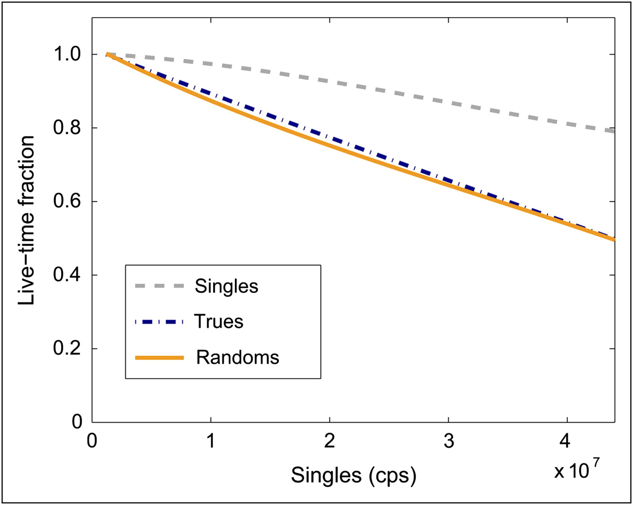
The object-independent live times as measured in the phantom study are shown in Figure 1. The singles live time is representative of count losses at the detectors. The trues and randoms live times are similar and fall at a greater rate than the singles. These coincidence live times represent the count losses at the detector, multiplexing losses within the coincidence electronics, and the application of the coincidence condition (9).

Live-time functions measured for Biograph-6 HiRez PET/CT scanner. cps = counts per second.
Extrapolated PS-NECR-A0 Curves
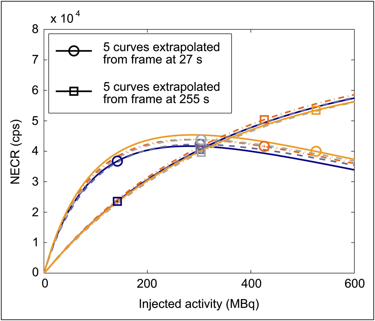
Examples of NECR-A0 curves extrapolated from the 5 injections to subject 3 are shown in Figure 2. Just 2 sets of NECR-A0 curves are shown, as generated from 2 different time frames; 1 set is from a frame during the tracer delivery phase (27 s, important for estimates of F), and the other frame is from the tracer washout period (255 s, important for estimates of VT). Within each frame, the variations between the 5 curves are small, with a similar CoV across the range of extrapolated activities. Between the 2 frames there are differences in both the maximum NECR and the value of A0 at which this maximum occurs. The curves originating from the earlier time frame in Figure 2 are more variable than those from the late time frame, as quantified in Figure 3, which shows the calculated mean CoV between the extrapolated curves as a function of the time frame from which the extrapolations pertain. These mean CoVs are calculated from 3–6 injections and as such are of low precision. The initial time frames, which cover the injection and soon after, have a larger CoV than do the later time frames. Once the tracer has cleared from the veins in the arm, the extrapolated curves are found to be in close agreement, with a CoV of less than 5% for most time frames (for subjects 2–6). All injections to subject 1 were given at the back of the wrist. The NECR extrapolations, estimated scatter fractions, and time–activity curves had greater variability between injections for this subject than for the 5 subjects injected at the antecubital fossa (data not shown).

For 2 time frames, 5 extrapolated NECR-A0 curves for subject 3 (with k = 2). The 2 sets of curves differ because of the combination of radioactive decay and change in distribution of activity within patient. Data points at 302 and 304 MBq are overlapping. cps = counts per second.
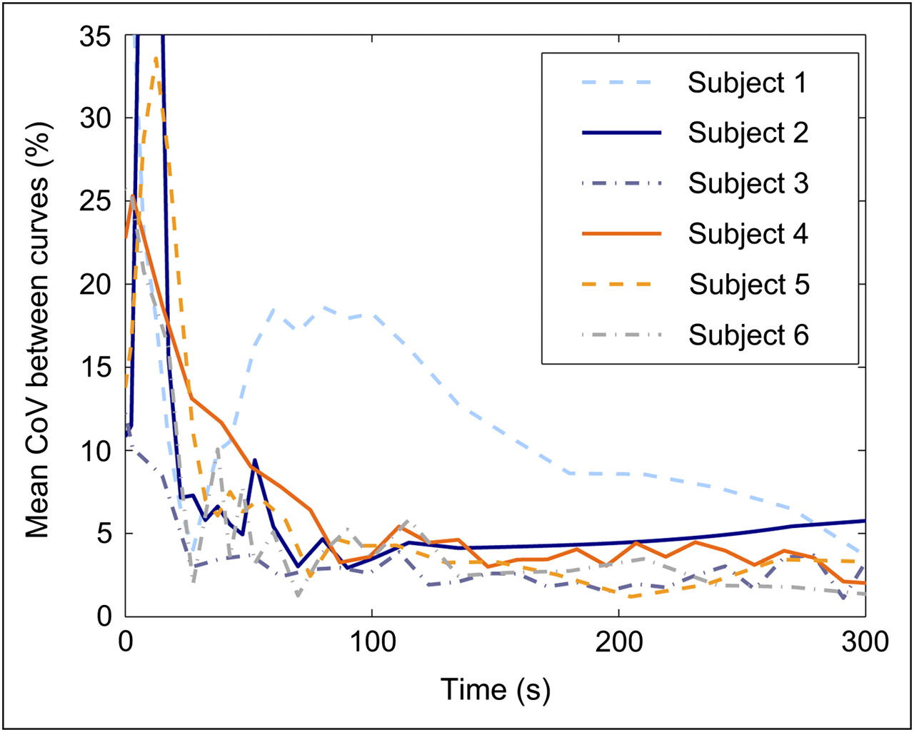
Mean CoV (%) between several extrapolated NECR-A0 curves that were generated for each patient and for each time frame. CoV was averaged between 40 and 750 MBq.
We found that the scatter correction scaling fails in the case of frames with few counts (<5.5 × 10⁵ net trues). This problem occurred regularly near the end of the scan in the case of short (12-s) frames (present in 6/21 scans) but was not observed in the case of variable-length framing (30 s at end of scan). With the exception of these final frames, the 2 frame sequences yielded similar counting rate data and scatter fractions.
Extrapolated PS-NECR Time Curves
Examples of NECR time curves, extracted from the NECR–A0–time surface generated for subject 4, are shown in Figure 4. Before 25 s, a large fraction of the activity is in the subject's arm, within the FOV. This produces a high NECR that falls as the tracer leaves the arm, before rising again when the tracer reaches the abdomen. For this subject, one sees that an A0 greater than 400 MBq will produce little or no change in the NECR during the tracer uptake period (important for estimates of F) but that it could improve the NECR at late time frames, during tracer washout (important for estimates of VT).
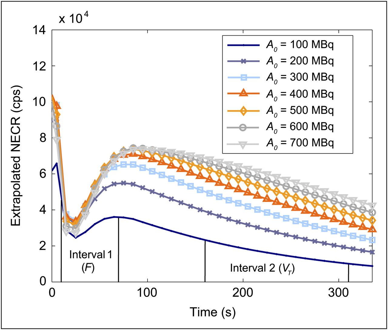
NECR time curves (k = 2) generated for subject 4, showing extrapolated NECR curves for different injected activities. The 2 intervals over which NECR was integrated are also shown (10–70 s and 160–310 s).
Estimates of Optimal Injected Activities
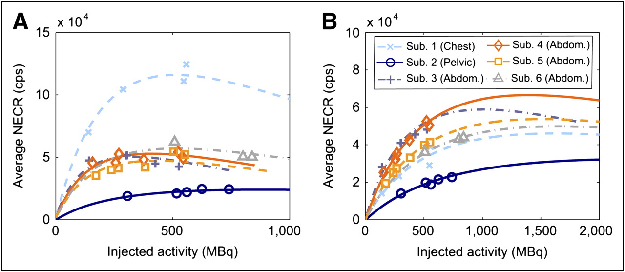
For each subject, the average NECR for the first time interval (10–70 s, F) is shown as a function of A0 in Figure 5A. The equivalent data for the second interval (160–310 s, VT) is shown in Figure 5B. The presented curves are the mean of the 3–6 curves, which originate from each injection. In Figure 6, these data are used to compare the relative changes in the SNR (given by  ) with A0, for which each time interval has been separately normalized to unity at the maximum SNR and for which the 4 subjects scanned at the abdomen have been averaged. The optimal A0's calculated from these data, that is, those that led to 95% NEC maximization, are shown in Table 2. For each subject, an optimal A0 was calculated from each injection and for each time interval (F and VT). Table 2 summarizes the mean and SD between injections for these optimal A0's. For abdominal (n = 4) and chest (n = 1) scans, we found optimal A0's of 15O-H2O in the range of 220–350 MBq for estimating F and 660–1,070 MBq for estimating the VT. Higher optimal A0's were found in the case of a pelvic scan (n = 1; 570 MBq for F and 1,530 MBq for VT). The maximum CoV of an optimal A0 calculated from the 3–6 NECR curves for a specific subject was 4.3% (subject 1, F). The mean CoVs for an individual's optimal A0's were 2.6% and 2.0% for the F and VT intervals, respectively. The optimal A0's for a specific subject, as derived from each injection, are thus in excellent agreement. Much larger deviations are seen to occur between different subjects.

Average NECR-A0 curves for each subject, as found by integrating NECR time curve over given time interval and dividing by duration of interval. (A) Results for interval 1 (F). (B) Equivalent results for interval 2 (VT). Measured values from each injection are shown as data points. Means of 3–6 extrapolated curves for each subject are shown as lines. abdom = abdomen; sub = subject.

Relative SNR for 2 time intervals (F and VT) and for 3 body areas scanned in this study. The 4 subjects scanned at abdomen were averaged for clarity. For each body region, curve that peaks first represents time interval 1 (F). Each time interval was separately normalized such that peak SNR is unity. sub = subject.
Estimated A0 for 95% NEC Maximization
Estimates of F and VT
The estimates of F and VT are shown in Figure 7. The estimates for each tumor are separately normalized to unity to show any correlation between the parameter estimates and A0. Data from subject 2 were discarded because of difficulties in extracting an image-derived input function from the external iliac arteries. The data from the low-activity injection (140 MBq) given to subject 1 were also discarded because the results of the kinetic fit were unstable. No significant correlation in the values of F or VT with A0 was observed with Pearson correlation coefficients equaling −0.18 and −0.27. The mean estimates of F for the tumors analyzed here ranged from 0.34 to 0.96 mL min−1 cm−3, with a mean across tumors of 0.62 mL min−1 cm−3. The same statistics for VT were 0.53–1.01 and 0.84 mL cm−3, respectively.
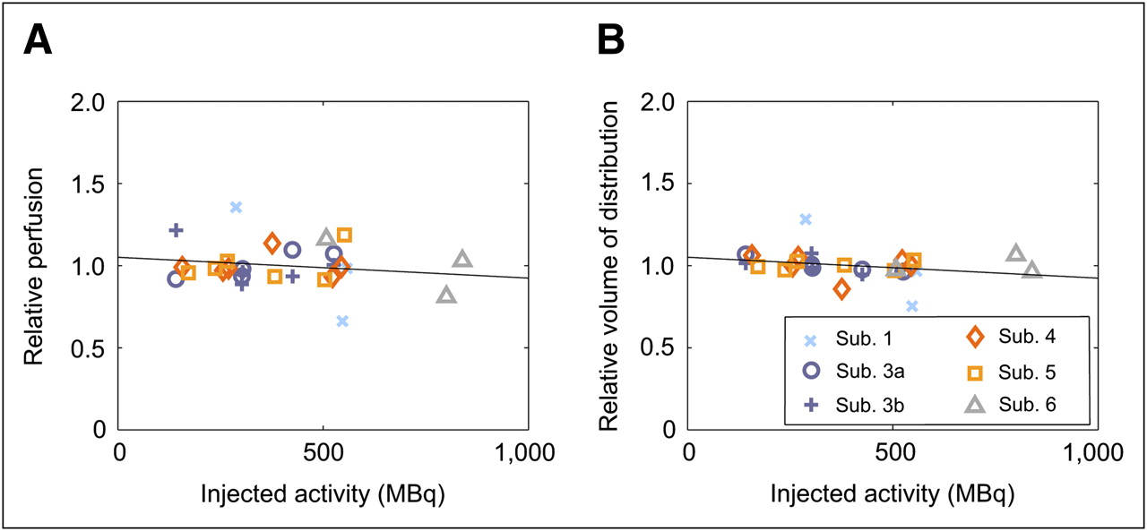
Estimates of F (A) and VT (B), separately normalized to unity for each tumor. Data show no systematic changes in F or VT with injected activity. Linear regressions (gradient, intercept) are equal at reported precision (−0.13 × 10⁻³, 1.05). Results from 2 distinct metastases are shown for subject 3. sub = subject.
DISCUSSION
We have shown how PS-NECR methods can be used to optimize the injected activity in dynamic PET. The data have also verified the accuracy of NECR extrapolations in the case of static imaging, in which the radiotracer is distributed throughout the subject's body. This verification comes from the good agreement between the extrapolations for all late time frames (Fig. 3). The optimal A0's for estimates of VT are 2.7–3.5 times greater than those for F. This is largely explained by the radioactive decay factor (2.9) between the 2 time intervals.
The variability between injections of the estimated optimal A0's (for a specific patient) was substantially less than the variability between subjects. Although this may cause difficulty in defining a single optimal A0 for a group of subjects based solely on their scan position and body size, examination of Figure 5 would suggest that one may inject a higher than optimal A0 without a substantial NEC penalty; conversely, if one injects a lower than optimal A0 there may be a large reduction in the average NEC. When estimating the optimal A0 for a prospective subject, it would thus be prudent to use an A0 that is toward the top end of the measured optimal A0's for the given subject size and scanning position. The penalty for such an approach is that some patients would receive a small increase in the effective dose of radiation without any increase (sometimes a decrease) in the total NEC. For example, an additional 200 MBq of 15O-H2O will result in an increase of approximately 0.2 mSv (18). Similarly, if one is interested in estimating both F and VT simultaneously, it would be reasonable to inject an activity that is greater than the optimal A0 for estimating F alone. Figure 6 allows the quantitative assessment of this compromise. Because the scanner used here maintains its ability to detect and record coincidences beyond the counting rate at which the peak NEC occurs, the compromise is acceptable. The point of intersection between the 2 curves (F and VT intervals) occurs within 6% of the maximum SNR in all cases.
It is worth reconsidering here the real aim of the optimization: to give more reproducible parameter estimates. Two questions arise: does NEC maximization imply maximization of the SNRIMG for the tumor, and does this maximization improve the reproducibility of the parameter estimates? The first question has been addressed by Watson, among others (9,19), who has shown that for FBP reconstruction, maximization of NEC increases the local SNR for almost all regions within an image. An exception to this rule was found in the large and high-activity region of the bladder (in an 18F-FDG scan), although global (95% maximum SNR) optimization of the injected activity still resulted in SNR optimization (>80%) for that region (9). The second question is more dependent on the methods used to estimate the parameters of interest, in particular the size of the ROI that is used to generate a time–activity curve. Increasing SNRIMG will improve the precision of parameter estimates in the case in which statistical noise in the time–activity curve is a limiting factor. In our experience, this is certainly the case for small ROIs (e.g., 2 mL) or in a voxelwise analysis.
Optimization methods based on the NEC do not consider the accuracy of images but simply their statistical noise. Because the injection of high activities can lead to errors in dead-time correction, care is required when determining A0. The requirement of accurate quantification in the early time frames (e.g., if using an image-derived input function) may limit A0, preventing maximization of the NECR for the later time frames. Such problems were not apparent in our data, however. Figure 7 shows no significant correlation between the parameter estimates and the injected activity.
Optimization of A0 in the case of OSEM image reconstruction should also be considered. The presented method is valid if maximization of the NEC also maximizes SNRIMG for the ROI, that is, the tumor. For OSEM this may not be true, because unlike FBP, the regional noise in an OSEM image is strongly correlated to the activity in that region (20). The optimal A0 is then dependent on the tumor uptake. However, in the absence of a better (tumor uptake–dependent) scheme for determining the optimal A0, maximization of the NEC is a reasonable approach for OSEM reconstructions. Future work is required to fully investigate the optimal A0 for OSEM reconstructions.
A possible limitation of the methodology is the use of a simple model for detector dead time. The model uses a single dead-time factor to describe dead time around the entire detector ring. This approximation may lead to errors during the initial time frames, for which most of the tracer is in the injection line and in the patient's arm. This highly asymmetric activity distribution, combined with the uncertainties in scatter correction for this distribution, may be the cause of inaccurate global counting-rate extrapolations for the initial frames. Another possible cause for the disagreement between extrapolations in the first few time frames is the variability in tracer delivery between injections. Although the rate of injection is well controlled, there is the possibility of physiologic changes between scans that could affect the blood flow (the total scanning time often exceeded 1 h). With the exception of the initial time frames, the counting-rate model is found to provide accurate predictions of the NECR as a function of the injected activity throughout the dynamic scan.
For moderate-sized subjects undergoing abdominal scans on this scanner, a standard A0 of 340 MBq of 15O-H2O is expected to produce a near-maximal NECR during the time frames that are most sensitive to changes in F. If estimating both F and VT from the same scan, an A0 of 600 MBq would be reasonable in terms of NEC maximization. However, this is somewhat dependent on the aims of the investigator and the significance that is placed in each of these parameter estimates. Initial data at other bed positions indicate that the optimal A0 for chest scans is similar to that found for abdominal scans but that pelvic scans are optimized at an increased A0 because of a lesser delivery and uptake of activity within the FOV.
Although multiple scans were acquired in this validation study, our data show that the optimal A0 can be estimated from a single scan for future subjects. For any patient undergoing repeated scans at the same position, it is possible to use the first scan to calculate a PS optimal A0 for the subsequent scans.
An extension to this optimization strategy would be to fully consider the biologic parameter–estimation process within the optimization rather than maximize the NEC over a representative time interval. However, the relative simplicity of the current method is one of its advantages, with the suggested extension beyond the scope of this work.
Although NEC optimization is a valid route for optimization of A0, it may be less useful for optimizing other aspects of scanning protocols, such as the site of injection. Changes in A0 do not affect the spatiotemporal distribution of the radiotracer and produce little or no change in the pattern of image variance. However, changes in the site of injection (for instance) may have a large effect on the spatiotemporal distribution of the radiotracer, which can lead to a change in SNRIMG for a given NEC and time frame (11).
CONCLUSION
PS-NECR extrapolation methods are valid when tested in human subjects and in dynamic PET. These extrapolations have been used to provide an estimate of the optimal injected activity in the case of 15O-H2O PET scans of the body, acquired in 3D mode.
The results of this work can guide future refinement and optimization of scanning methods and protocols for 15O-H2O scans on modern whole-body LSO-based PET cameras. The generic method of optimizing the injected activity may also be applied to other scanners and radiotracers.
Acknowledgments
We thank Charles Watson, Bernard Bendriem, Lars Eriksson, and Hartwig Newiger of Siemens Medical Solutions for their useful comments and support. We also thank the operational staff at WMIC for their help in data acquisition, Rainer Hinz for many helpful discussions, and Juan Valle for his help in patient recruitment. This work was supported in part by a studentship from Siemens Medical Solutions and was funded in part by Cancer Research U.K. (grant 153/A4331) and the U.K. Department of Health (Experimental Cancer Centre grant).
Footnotes
-
COPYRIGHT © 2009 by the Society of Nuclear Medicine, Inc.
References
- Received for publication January 30, 2009.
- Accepted for publication May 22, 2009.


Jump to section
Related Articles
Cited By...
- No citing articles found.