


Abstract
PET was used to measure tumor blood flow, which is potentially valuable for diagnosis and assessing the effects of therapy. To help visualize regional differences in blood flow and to improve the accuracy of region-of-interest placement, a parametric imaging approach was developed and compared with the standard region-of-interest method. Methods: Five patients with renal cell metastases in the thorax were studied using [15O]water and dynamic PET. To assess the reproducibility of the blood flow measurements, multiple water studies were performed on each patient. Model fitting was done on a pixel-by-pixel basis using several different formulations of the standard single-compartment model. Results: The tumors studied spanned a wide range of blood flows, varying from 0.4 to 4.2 mL/min/g. These values were generally high compared with those of most other tissues, which meant that the tumors could be readily identified in parametric images of flow. The different model formulations produced images with different characteristics, and no model was entirely valid throughout the field of view. Although tumor blood flow measured from the parametric images was largely unbiased with respect to a standard regional method, large errors were observed with certain models in regions of low flow. The most robust model throughout the field of view had only 1 free parameter and, compared with a regional method, gave rise to a flow bias of 0.3% ± 3.1% for tumor and 16% ± 11% for low-flow soft tissue (muscle plus fat). With this model, tumor blood flow was measured with an SD of 7.6% ± 4.0%. Conclusion: Parametric imaging provides a convenient way of visualizing regional changes in blood flow, which may be valuable in studies of tumor blood flow.
Information regarding tumor perfusion is potentially valuable for diagnosis, for assessing the expected delivery of anticancer agents, and also for monitoring the effects of therapy. PET, in conjunction with [15O]water, has been used extensively to measure blood flow in the fields of neurology (1,2) and cardiology (3,4), but the technique has not been widely applied in oncology. Many of the reported tumor applications have been confined to the brain (5–7), although studies of liver (8,9), colorectal (10), and breast (11) carcinoma have also been performed. A range of different acquisition and analysis techniques has been used to investigate tumor blood flow and, in some cases, methodological restrictions limited these studies to a semiquantitative approach.
In this study we used a dynamic acquisition protocol that, in conjunction with appropriate kinetic models, enabled the quantitative measurement of tumor blood flow. The standard method for analyzing such data (which we refer to as the region-of-interest [ROI] method) is to draw an ROI around the tumor, generate a time–activity curve from this region, and then apply a kinetic model to the time–activity curve to measure flow and other parameters described by the model. One of the problems with the ROI method is that each time a new region is to be analyzed, the entire set of dynamic data must be used to produce the time–activity curve. If large numbers of regions are to be analyzed, this produces equally large numbers of time–activity curves, and the resulting data are often difficult to present in a meaningful manner. In addition, identification of the tumor ROI is not trivial and, even if additional information is available from other modalities, the definition of ROIs may be prone to errors. Finally, most blood flow models assume that blood flow is uniform throughout the tumor ROI, which may not be true. To help overcome these problems we have developed a parametric imaging approach in which the model fitting is performed on a pixel-by-pixel basis, resulting in images that directly reflect regional blood flow. Parametric images have been used widely in studies of cerebral blood flow with [15O]water (12–15) and also in other studies of the brain—for example, with [11C]flumazenil (16) and [18F]fluoro-l-dopa (17). The technique has also been used in cardiac studies with FDG (18), renal studies with [13N]ammonia (19), and tumor studies in the liver with FDG (20).
The application of the parametric imaging technique to tumor blood flow studies using [15O]water raises several interesting issues. Although the kinetic model used in most water studies is a standard single-compartment model, several different variations to this model have been developed, each of which has its own advantages in different situations. In studies of the brain, a formulation of the model that is frequently used allows measurement of both flow and volume of distribution. This formulation derives flow information primarily from the influx phase of the dynamic data and is well suited to brain studies in which organ motion can be minimized. In studies of the heart, however, there can be significant partial-volume effects caused by motion of the myocardium and by the fact that the myocardial thickness (typically ≤10 mm) is comparable with the resolution of most PET scanners. An alternative formulation of the model used for cardiac studies (21) assumes that the volume of distribution in the myocardium is known and permits flow to be computed in such a way that it is, in principle, independent of partial-volume effects. This formulation derives flow from the efflux phase of the dynamic data. In addition, so-called spillover terms are often introduced into the model to account for contamination of the tissue time–activity curves by activity in nearby blood vessels.
The optimum formulation of the blood flow model for the measurement of tumor perfusion has not been established. Therefore, in this study, which concentrates on methodological issues, we examined the characteristics of 6 different formulations of the standard [15O]water blood flow model. We estimated the reproducibility of the kinetic parameters derived from each of these formulations using data from repeated flow measurements. Finally, we examined the quantitative accuracy of the parametric images by comparing tumor blood flow values from these images with those obtained using the standard ROI methodology. These issues may prove to be particularly important in light of the development of new anticancer drugs that aim to affect tumor angiogenesis (22).
MATERIALS AND METHODS
Patients
Studies were performed on 5 patients with renal cell metastases who were known, by previously acquired CT and MRI, to have lesions that measured >2 cm in diameter. This group consisted of patients in whom both the tumor and the heart (used for the noninvasive determination of the arterial input function) could be imaged simultaneously by the PET scanner. Before enrollment in the study, each patient gave informed consent for the procedure, which had been approved by the institutional review board of the National Cancer Institute.
Data Acquisition
Image data were acquired on an Advance PET scanner (General Electric Medical Systems, Milwaukee WI) (23) that was operated in septa-extended, 2-dimensional mode. Thirty-five transaxial planes of data were acquired simultaneously with a slice-to-slice distance of 4.25 mm. Data acquisition started immediately before a peripheral intravenous injection of 1.85 GBq [15O]water that was administered as a rapid bolus over ∼5 s. Each acquisition lasted for 5 min and was performed in a dynamic mode with the following frame times: 20 × 3 s, 6 × 10 s, and 6 × 30 s. To assess the reproducibility of the perfusion measurements, each patient had either 2 or 3 separate [15O]water studies. These studies were performed either on a single day or over 2 consecutive days.
All projection data were corrected for photon attenuation using data derived from an 8-min transmission scan that was acquired immediately before tracer administration. The transmission scans were acquired with septa extended using 2 rotating 68Ge rod sources that had a total activity of 333–555 MBq over the period during which the scanning was performed. The emission data were scatter corrected (24), and images were reconstructed using filtered backprojection with a transverse spatial resolution of ∼7-mm full width at half maximum (FWHM) at the center of the field of view. To suppress noise and thus reduce the variability of the parameter estimates in the subsequent model fitting, the images were resampled so as to have a 4 × 4 mm pixel size, and an additional smoothing filter was applied in the transaxial plane. This resulted in a spatial resolution at the center of the field of view of ∼14-mm FWHM in the transaxial plane and ∼4-mm FWHM in the axial direction.
Both MRI and FDG PET data were available for qualitative comparison with the flow images. After the last [15O]water study, the patient remained within the PET scanner and was injected with 555 MBq FDG. Forty-five minutes after injection, an additional 15-min emission scan was begun. The resulting FDG data were processed in the same way as the [15O]water data, although no additional smoothing was applied after reconstruction. T1-weighted, contrast-enhanced MR images, acquired on a 1.5-T unit (Signa; General Electric Medical Systems), were also available.
Parametric Images
[15O]Water is a chemically inert, freely diffusible tracer, and its behavior in tissue can be described by the following equation (25,26):
 Eq. 1where C(t) is the radioactivity concentration in tissue at time t; Ca(t) is the radioactivity concentration in arterial blood at time t; f is regional blood flow (per gram of perfused tissue) from plasma to tissue; Vd is the volume of distribution for water, which is defined as the ratio of the water concentration in tissue to that in blood at equilibrium; and ⊗ denotes convolution. The limited spatial resolution of the PET scanner means that measurements of tissue activity concentrations may be biased because of the partial-volume effect. In addition, the tissue activity curve may be contaminated by arterial blood from vessels nearby or within the volume of interest. To compensate for these 2 effects, one can incorporate a partial-volume factor into Equation 1 and add an additional spillover term proportional to the arterial blood activity concentration, producing the following expression:
 Eq. 2where Ci(t) is the tissue activity concentration measured from the PET image, α is the corresponding recovery coefficient, and Va is the fraction of the arterial blood concentration that appears in the tissue. Note that spillover is assumed to be proportional only to the arterial activity concentration, although in certain regions venous blood may dominate and this assumption will be in error.
α, f, Vd, and Va are, in general, unknown parameters to be determined by least-squares estimation. A unique solution for all 4 parameters cannot be obtained simultaneously, and this fact, plus noise constraints, means that it is necessary to reduce the number of free parameters in the fit. There are several ways to reduce the number of parameters, each of which requires slightly different assumptions. Table 1 summarizes the parameter assumptions for the 6 different formulations of the model that were considered. Model 1a derives f from the influx term (α × f) and Vd from the efflux term (f/Vd), with the assumption of perfect resolution recovery. Model 2a makes an assumption about the volume of distribution and derives f from the efflux term, which is independent of partial-volume effects. Note that models 1a and 2a are essentially the same with the flow information being obtained from different terms. Model 3a makes assumptions about the recovery coefficient and volume of distribution but calculates flow from both the influx and efflux parts of the curve. Models 1b, 2b, and 3b are identical to models 1a, 2a, and 3a but also include an arterial blood volume term that is proportional to the arterial input function. For those models in which Vd was fixed (models 2a, 2b, 3a, and 3b), we assumed a value of 0.91 mL/g, which is frequently accepted for the myocardium (21). Of course, this value may not be applicable for other tissues, and the validity of this assumption will be examined.
Six Formulations of Standard [15O]Water Blood Flow Model
The models were fit to the dynamic water data on a pixel-by-pixel basis, resulting in 1 or more parametric images (1 for each free variable in the model). Parameter estimation was performed using the rapid linearized least-squares search method of Koeppe et al. (14), which involved precomputing the convolution of the input function with exp(−k × t) for a range of k values. The parameters that minimized the total squared discrepancy between the measured data and the model (χ2) were obtained by recursively evaluating χ2 at 3 points over the k range, with the distance between each sample becoming progressively smaller. On the basis of expected flow values, the search was initially performed over the k range from 0 to 1 per minute, although if a minimum was found toward the top of this range the search was expanded to cover 0–10 per minute. A total of 2561 discrete k values were evenly sampled from 0 to 10 per minute, which, for a volume of distribution of 0.91 mL/g, resulted in flow intervals of 0.00355 mL/min/g. Fitting was performed in a weighted manner with each time frame having a weight that was inversely dependent on the variance of the image data. This variance was estimated by an approximate formula that was a function of the frame duration, scanner dead time, and the number of counts in both the prompt and delayed coincidence windows. High randoms and dead time at the start of the study, combined with short-acquisition frame times, meant that early frames were often weighted less heavily than later ones. The image dimensions were 128 × 128 and, to speed up the computation, the transmission image was used to mask out pixels that were in the surrounding air. The computation time to produce 35 slices of parametric image data for a single model was ∼10 min on a VAX 4000 computer (Digital Equipment Corp., Maynard, MA).
The input function Ca(t) was estimated from the image data using manually defined ROIs drawn in the left atrium. Frames 5–12 (total acquisition time, 24 s) of the dynamic water data were added to give an average image of the early phase of the study that clearly showed the blood pool. Irregularly shaped ROIs with a mean size of 4.4 ± 2.4 cm2 per slice were drawn in the left atrium in 4 adjacent planes. These ROIs were then applied to the corresponding dynamic images before the additional postreconstruction smoothing filter (and therefore at a spatial resolution of ∼7-mm FWHM). For each frame the mean activity concentration within the volume formed by the 4 ROIs produced an approximate, noninvasive arterial input function.
Image Analysis
The quantitative nature of the parametric images was assessed by ROI analysis. Although tumor blood flow was the main interest of the study, ROIs were drawn around regions of myocardium and soft tissue as well as tumor. The myocardium was of interest because it has been widely studied and provided an opportunity to compare the quantitative values obtained from the parametric images with previously published data. The soft-tissue regions were useful because they showed the typical flow values that might surround a tumor and they also highlighted the noise problems that occur in regions of low flow. Each ROI was manually drawn using the model 3b flow images from each patient's first water study. To compensate for patient motion between scans, the original ROIs were visually repositioned, but not redrawn, for the subsequent studies performed on the same patient. Tumors were identified in conjunction with the FDG data and ROIs (mean size, 6.5 ± 3.0 cm2 per slice) were drawn, in 3 adjacent planes, around the region of highest flow. Similarly, the myocardial ROIs (mean size, 21.1 ± 5.1 cm2 per slice) were defined in 3 transverse planes and included the septum, anterior wall, and lateral wall. The soft-tissue ROIs (mean size, 60.8 ± 24.2 cm2) were drawn in single planes and probably included a combination of pectoral muscle and fat.
The ROIs described above were applied to the parametric images for each model. The mean flow within each ROI was calculated and, in the cases of the tumor and myocardial regions, the data from multiple planes were averaged to obtain the mean flow over the volume of interest. Because an independent gold standard was not available, the mean flow values from the parametric images were compared with flows measured using the standard ROI method. The ROI method computed flow by applying the same ROIs to the dynamic water data and then fitting the resultant time–activity curves to each of the 6 models, using previously reported nonlinear regression software (27). Input functions and weights used for the ROI method were identical with those used for the pixel-by-pixel method. Therefore, the 2 methods should differ only because the mean of the individual pixel flows may not equal the flow from the mean time–activity curve from all individual pixels (especially if flow is not homogeneous throughout the ROI) and because of possible differences in the fitting algorithm.
RESULTS
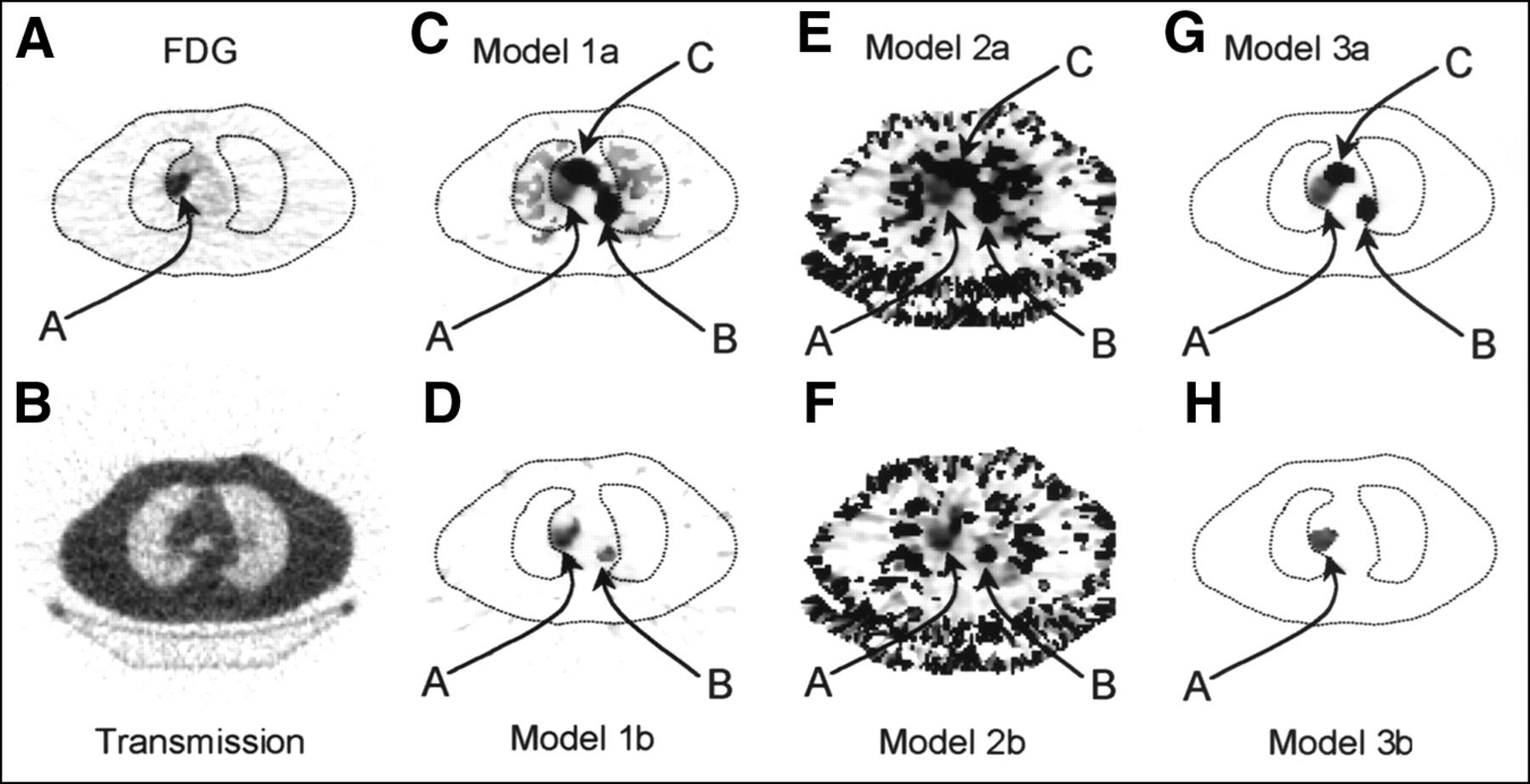
Figure 1 shows an example of the blood flow parametric images for each of the 6 models. Corresponding FDG and transmission images for the same patient (patient 3) are also shown for comparison. Note that the tumor can be seen as a region of high FDG uptake that corresponds to an area of increased blood flow in each of the 6 flow images. Note also the different noise structure of the 6 flow images, particularly the high-intensity pixels toward the edge of the patient in the model 2a and 2b images. With models 1a, 2a, and 3a, which do not include a blood volume term, blood vessels appear as regions of high flow. Adding an arterial blood volume term to models 1a, 2a, and 3a resulted in the formulations of models 1b, 2b, and 3b. This addition had the effect of removing much of the arterial blood from the flow images. For example, compare Figure 1C with Figure 1D, Figure 1E with Figure 1F, and Figure 1G with Figure 1H. The arterial curve from the left atrium was used for the blood volume term in models 1b, 2b, and 3b. No corrections were made for delay or dispersion because these effects will be different at different points in the body, and the data were too noisy to include them as additional parameters in the fit. As a result, venous blood, or arterial blood that was significantly delayed with respect to the heart, was not well described by this term, and blood vessels occasionally remained in the perfusion images as regions of high flow (Figs. 1D and F).

Representative FDG, transmission, and flow images of patient 3 show nature of parametric images derived from each of 6 models. (A) FDG. (B) PET transmission. (C) Flow f, model 1a. (D) Flow f, model 1b. (E) Flow f, model 2a. (F) Flow f, model 2b. (G) Flow f, model 3a. (H) Flow f, model 3b. Arrow A indicates tumor; arrows B and C indicate aorta. Images in (A) and (B) were acquired sequentially with water data and are approximately aligned with parametric images. Patient outline obtained from transmission image has been superimposed on images in (A), (C), (D), (G), and (H) to aid interpretation. Images in (A) and (B) were scaled to their individual maximums; images in (C–H) were scaled from 0 to 5 mL/min/g, and pixels with flows that exceeded upper limit took maximum color table value.
The effect of adding a blood term to model 3a can also be seen in Figure 2 for another patient. The aorta, which appeared as a high-flow region in Figure 2C, was removed from the flow image in Figure 2E. Figure 2F shows the arterial blood volume image that corresponds to the flow data in Figure 2E. In this image, high blood contributions can be seen in the aorta (Va = 0.94) and, to a lesser extent, the lungs (Va = 0.25). Tumor A can be clearly seen as an area of high FDG uptake in Figure 2A and also shows high perfusion in the flow images (Figs. 2C and E). Note that in the FDG image, the presence of a second lesion was also suspected in the right lung, although additional information would increase confidence in this assessment. In Figures 2C and E, lesion B is more strongly suggested, and the flow images can be seen to provide information that complements the metabolic data. The MR image, shown in Figure 2D, confirmed the presence of a suspicious lesion.
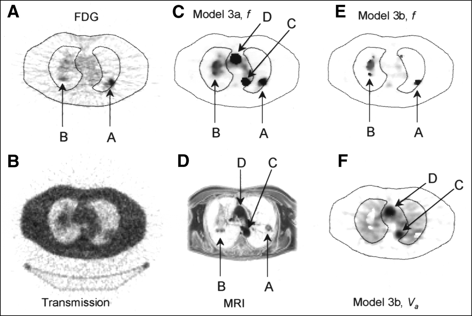
Example images of patient 1. (A) FDG. (B) PET transmission. (C) Flow f, model 3a. (D) MRI. (E) Flow f, model 3b. (F) Arterial blood volume Va, model 3b. (A and B) Images were acquired sequentially with water data and are approximately aligned with parametric images. (D) MR image shows approximately same region as PET images. Arrows A and B indicate lesions; arrows C and D indicate aorta. Patient outline obtained from transmission image was superimposed on images in (A), (C), (E), and (F) to aid interpretation. Images in (A), (B), (D), and (F) were scaled to their individual maximums; images in (C) and (E) were scaled from 0 to1 mL/min/g, and pixels with flows that exceeded upper limit took maximum color table value.
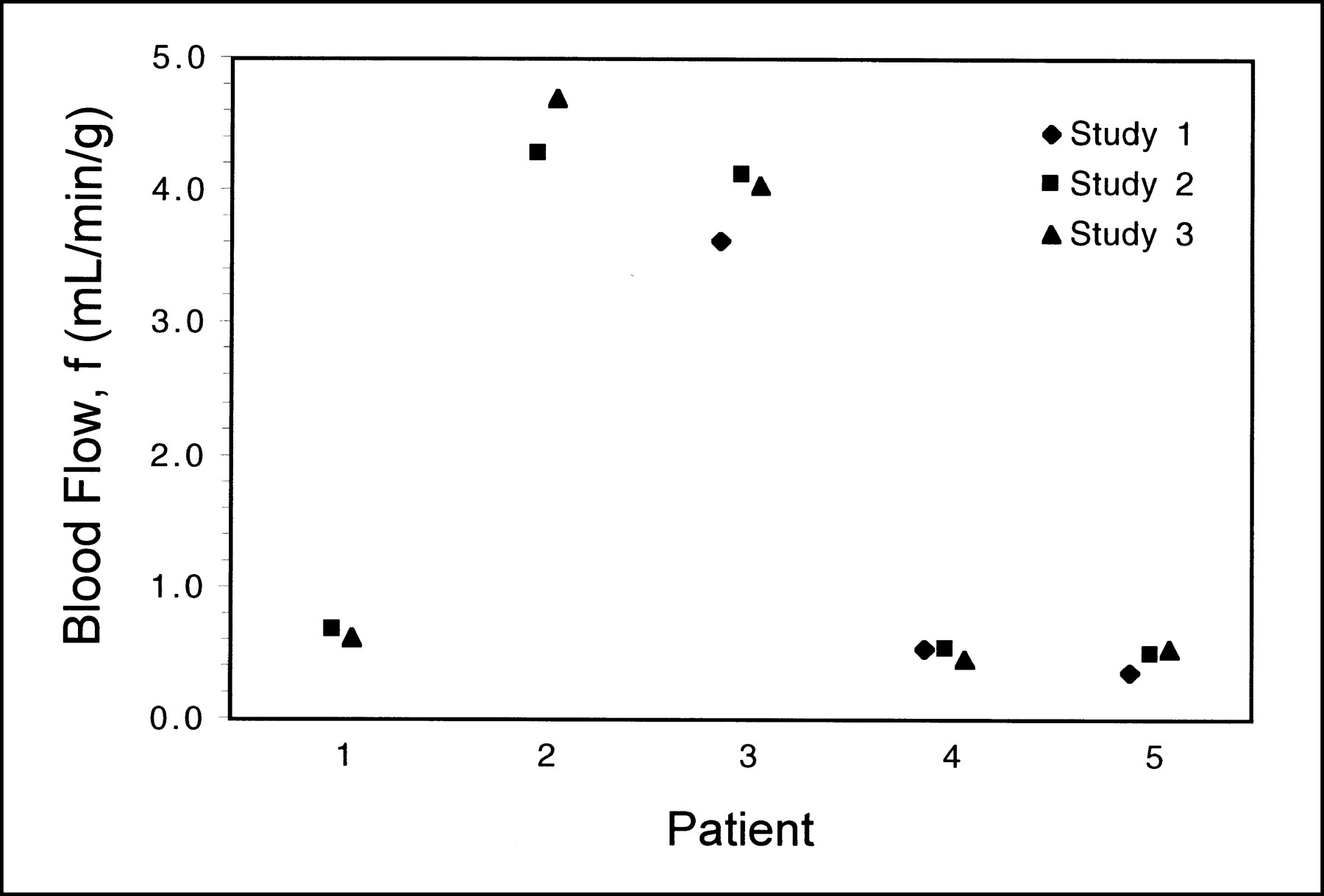
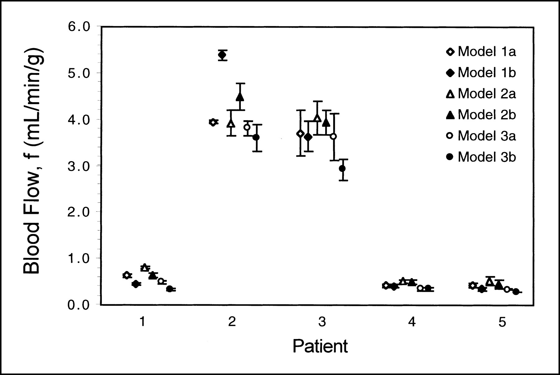
Figure 3 shows the reproducibility of tumor blood flow measured from the parametric images (with model 2b, in this case), for each of the 5 patients, as determined from the 2 or 3 replicate measurements. The 5 tumors studied spanned a very wide range of blood flows, varying from 0.4 to 4.2 mL/min/g, and the replicate studies are seen to give fairly consistent flow values. Figure 4 shows the mean tumor blood flow (averaged over the 2 or 3 replicates) for each patient and model. The error bars denote 1 SD, as estimated from the replicate studies. Comparing the flows from model 1a to model 1b, model 2a to model 2b, and so forth, the effect of adding the blood term can be seen. Addition of the blood spillover term reduced the tumor flow, on average, by 2.4% (model 1a to model 1b), 4.7% (model 2a to model 2b), and 15.0% (model 3a to model 3b). To compare the variability of the different models, each of these SDs of flow were divided by their respective means to determine a series of normalized SDs. The mean of these normalized SDs, for all patients, were 7.2% ± 4.8%, 7.4% ± 3.5%, 8.8% ± 5.6%, 10.1% ± 6.4%, 7.6% ± 4.0%, and 6.6% ± 3.2% for models 1a, 1b, 2a, 2b, 3a, and 3b, respectively. Note that the normalized SDs are small and are not significantly different between models (Student paired t test, P > 0.28 in each case).

Multiple tumor blood flow measurements obtained from model 2b parametric images. Patients 1 and 2 each had 2 water studies; patients 3–5 each had 3 water studies.

Tumor blood flow for each of 5 patients calculated from parametric images. Results from 6 different formulations of single-compartment model are shown, slightly offset from each other. Blood flow values are mean of measurements obtained from separate water studies, and error bars denote 1 SD.
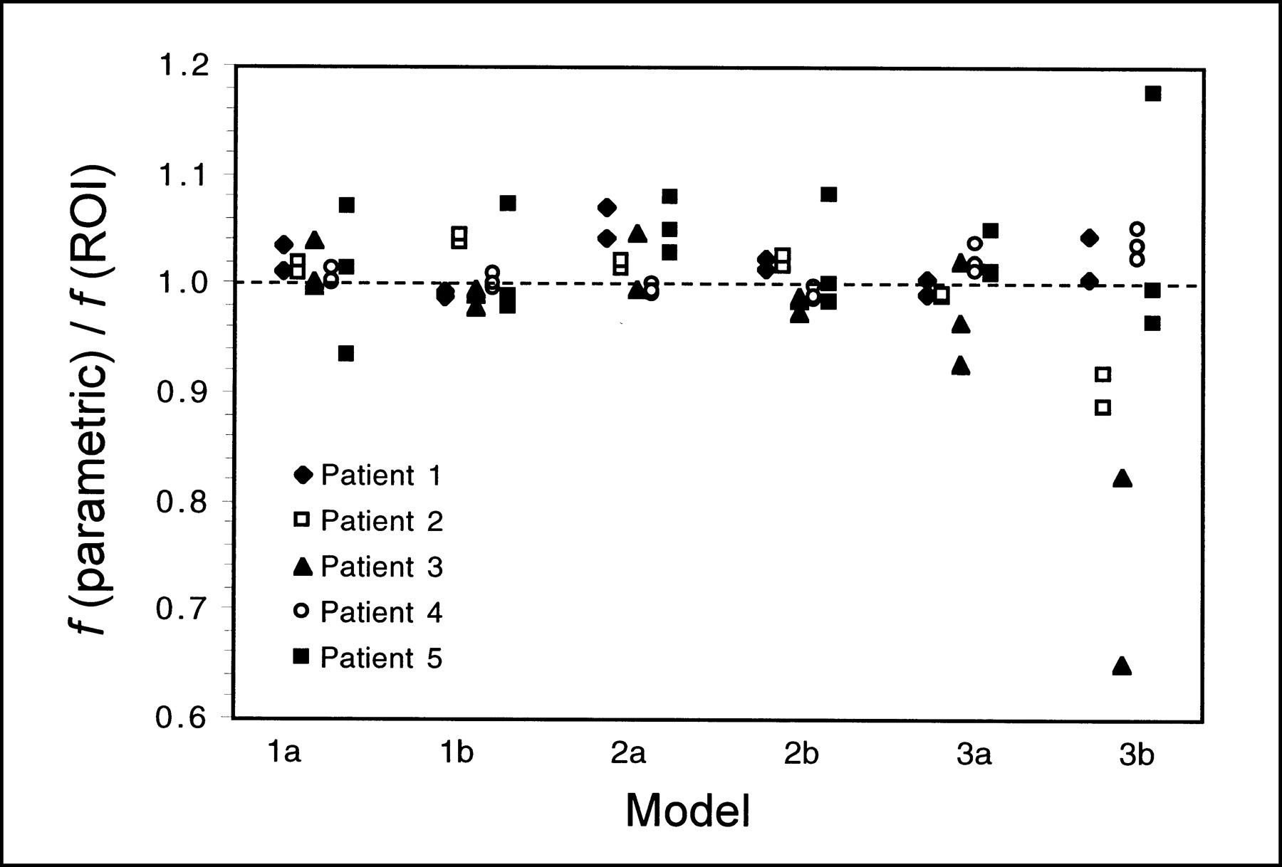
The tumor flow data obtained from the parametric images, shown in Figure 4, were compared with the equivalent data obtained using the ROI method. Figure 5 shows the parametric flow values divided by the ROI flow values for each patient and model (a value of 1 indicates perfect agreement between the 2 methods). The mean ± SD (over all patients and studies) of these fractions were 1.012 ± 0.031, 1.006 ± 0.029, 1.026 ± 0.030, 1.006 ± 0.029, 1.003 ±0.031, and 0.942 ± 0.155 for models 1a, 1b, 2a, 2b, 3a, and 3b, respectively. Only for model 3b did the ROI and parametric methods give appreciably different mean flow values. Furthermore, only for this model were there individual patients who exhibited large differences in flow between the 2 methods (maximum difference, 35%).

Tumor blood flow calculated from parametric images as fraction of same parameter calculated using ROI method with corresponding model. Data for 6 models are shown and, for each model, data points for each patient are offset for clarity.
For each patient, the soft-tissue ROIs were assumed to encompass tissues with comparable blood flow. The mean and SD of the flow measurements were thus calculated from the 13 studies performed on all patients. These data, which were calculated separately for each model, are shown in Table 2 for both the parametric image and the ROI methods. Note the range of flows given by the different models and the large differences in the flow obtained by the 2 methods for models 1a, 1b, 2a, and 2b. Note also the closer agreement between the parametric and ROI data for models 3a and 3b.
Soft-Tissue Blood Flow Calculated Using Both ROI and Parametric Image Methods
Values of the volume of distribution for water, obtained using the parametric images and the ROI method, were compared for both soft-tissue and tumor regions. Table 3 shows the mean values for all patients, calculated using model 1b. On average, the estimates of the volume of distribution for tumor were very similar (Student paired t test, P = 0.57) for the 2 methods; furthermore, no individual patients differed by >3%. Note the large discrepancy between the parametric image and ROI data for the soft-tissue regions that was highly significant (Student paired t test, P < 0.001).
Volume of Distribution for Regions of Tumor and Soft Tissue
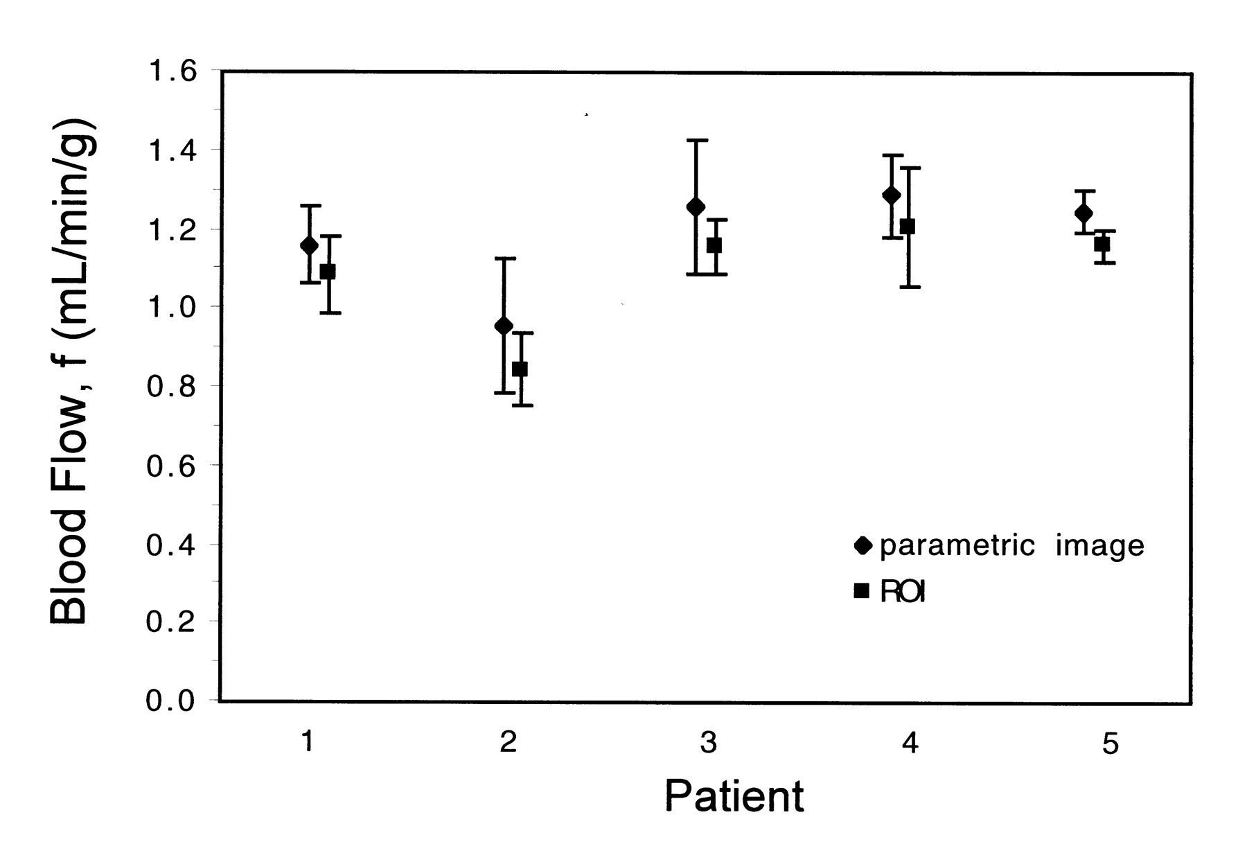
The values of myocardial blood flow obtained from the parametric images were compared with those measured by the ROI method using, in each case, model 2b. The absolute values of flow obtained by this latter method have been well validated for the myocardium (21). Flow values calculated using both ROI and parametric image methods are shown in Figure 6. The mean blood flow was 1.18 ± 0.13 and 1.09 ± 0.15 mL/min/g for the parametric and ROI methods, respectively; on average, the parametric images overestimated flow by 8.5% ± 2.8% compared with the ROI method. Note that all 5 patients had myocardial blood flow in a similar range, including patients 2 and 3, who had large values of tumor blood flow (Fig. 4).

Myocardial blood flow obtained using both parametric image and ROI methods for each patient. Model 2b was used in both cases and data points for each patient have been offset for clarity. Blood flow values are mean of measurements obtained from separate water studies, and error bars denote 1 SD.
DISCUSSION
The particular tumors encountered in this study had blood flow in the range 0.4–4.2 mL/min/g and, compared with the low values typically found in surrounding tissue, this meant that they could be readily identified on the parametric flow images. In Figure 1, the tumor can be seen on the parametric images from each of the flow models as a region of locally increased perfusion that corresponds to the area of high FDG uptake. The parametric maps may facilitate comparisons between blood flow and FDG metabolism and might be useful in studies of tumor heterogeneity. In regions with low blood flow, the fits frequently failed to reach an accurate convergence (described below), and the images appeared noisy. This effect was most pronounced in the images produced with models 2a and 2b and made these images hard to interpret. Model 3b handled the low-flow regions well but displayed sharp discontinuities at high-flow areas that were not present in the model 3a images. Having only 1 free parameter, model 3a was robust throughout the field of view and, apart from the arterial blood volume effects, produced the most easy-to-interpret flow images.
The tumor blood flow obtained from the parametric images compared well with the corresponding data derived from fitting the model to the regional time–activity curves (Fig. 5). Although differences in the results of the 2 approaches might be expected because of tissue heterogeneity (28), no significant differences were detected for models 1a, 1b, 2a, 2b, and 3a. The reason for this close agreement is probably associated with the fact that the image data were heavily smoothed and the pixels within the tumor regions were thus highly correlated. It may be possible to reduce the size of the transverse smoothing filter if the injected dose were increased, if additional smoothing were applied in the axial direction, or if an iterative reconstruction algorithm were used. For model 3b, the discrepancy in the flow results may be attributed to the incorrect assumptions of this particular model (i.e., that resolution recovery is perfect and that the volume of distribution is fixed at 0.91 mL/g). Including a blood term in this model provided a mechanism to artificially compensate for the differences between the measured data and the model, but the accuracy of the parameter estimates was apparently compromised. The large variability in ROI versus parametric flow values seen in Figure 5 for model 3b may be caused by the increased sensitivity of this model to the high noise levels present in the pixel-by-pixel data. Errors of this sort may be more likely to occur in regions of high flow where the tissue time–activity curve more closely resembles the input function. This problem can be visualized in the model 3b images (Figs. 1H and 2E) as a sharp discontinuity between high and low flow, which was not consistent with the 14-mm resolution of the image data. The quantitative accuracy of these images may not be reliable in these regions, but the sharp discontinuity did provide a way of identifying the high-flow part of the tumor that was used for ROI definition. Note that the invalid model assumptions described above also affect model 3a, but, because this model has only 1 free parameter, it may handle these data better. Although models 1b and 2b also include a blood volume factor, these models allow the influx and efflux terms to be independent free variables and the problem does not arise.
Although estimates of tumor blood flow obtained from the parametric images were unbiased (at least for models 1a, 1b, 2a, 2b, and 3a) with respect to the ROI method, this was not the case for other regions of the image. For nontumorous soft tissue, column 4 of Table 2 shows that the parametric images gave estimates of flow that were considerably greater than those of the ROI method, particularly for models 2a and 2b but also for models 1a and 1b. The high flow encountered in the tumors resulted in both pixel and ROI time–activity curves with relatively low noise, which meant that reasonable fits were achieved. For other parts of the body, the blood flow was lower and the time–activity curves, particularly for the parametric method, were much noisier. This led to model parameters with relatively high variance, especially in the case of models 1a, 1b, 2a, and 2b, which had 2 or 3 free parameters. In our implementation of the parametric method, model parameters were always computed, although noisy data tended to produce k values (14) toward the maximum of the permitted search range (these points are readily apparent in Figs. 1E and F). Even when the search algorithm was replaced by a brute-force search that examined all k values in the permitted range, the problem remained. This effect is equivalent to a failure to converge (when the influx is low it is difficult to measure the efflux) and accounts for the very high flow values encountered in the soft-tissue regions of the parametric images (for models 1a, 1b, 2a, and 2b).
For the soft-tissue data obtained with models 3a and 3b, good agreement can be seen between the ROI and parametric imaging results (Table 2). This is because these models imposed a more constrained fit and, in all cases, reached convergence. Although these ROIs probably contain a mixture of muscle, fat, and other soft tissue, the flow values agree well with previously reported muscle blood flow values of 0.018 ± 0.010 mL/min/g (29). The flow values obtained with the ROI method for models 1a and 1b are also consistent with these previously published values, but the flow values for models 2a and 2b are an order of magnitude greater. This is associated with the fact that, in these models, an assumption was made about the volume of distribution. The flow information comes entirely from the washout term and, although this value is expected to be largely independent of partial-volume effects, it requires that the volume of distribution be known. For the myocardium, this value is thought to be 0.91 mL/g, but it is not likely that this value is applicable throughout the body. From model 1b we can estimate the volume of distribution, and the data in Table 3 show a value of 0.123 ± 0.039 mL/g (ROI method) for soft tissue. Taking Vd = 0.91 mL/g was therefore a poor approximation, in this case, and might account for the errors in the soft-tissue flow data obtained with these models. For the tumor regions, the volume of distribution was found to be 0.80 ± 0.15 mL/g and 0.79 ± 0.14 mL/g for the parametric image and ROI methods, respectively. These values may be underestimates (30) of the true values because of partial-volume effects, and it seems that the assumed value of 0.91 mL/g might be more accurate for these tumors than for soft tissue. Of course, other tumors may have quite different volumes of distribution, in which case models that do not fit Vd would be incorrect. Further studies involving a larger group of tumors would be required to verify this.
In one of the few quantitative studies of tumor blood flow (11), values of flow in malignant lesions were found to be 0.298 ± 0.170 mL/min/g. This study was of breast tumors, and flow was calculated using the model that we have referred to as model 1a. At least 2 of the 5 patients in our study had values of tumor blood flow that were significantly greater than this value: approximately 4.2 and 3.6 mL/min/g. Although these values seem surprisingly high, it should be remembered that renal cell metastases are known to be very vascular tumors. In addition, the flow in other parts of these images was in the normal range, suggesting that the high-flow values for tumor are reliable. The mean myocardial blood flow for all 5 patients, obtained with model 2b (the model typically used for cardiac studies) was 1.18 ± 0.13 and 1.09 ± 0.15 mL/min/g for the parametric and ROI methods, respectively. All 5 patients were expected to have normal myocardial flow, and our data, including the 2 patients with the high tumor flows, were consistent with previously reported normal values of 0.95 ± 0.09 mL/min/g (21), obtained using the same model. The pixel-by-pixel method overestimated flow by 8.5% ± 2.8% compared with the ROI method. This is not unexpected. The pixels near the edge of the myocardium had very low counts and resulted in flow values that had large relative SDs. Because the lowest possible flow value was 0 and the highest was (arbitrarily) 10, averaging such noisy pixel values together would bias the flow data to slightly high values. This effect does not occur with the ROI method because the pixels with the low counts do not contribute significantly to the mean time–activity curve.
In this study, the parts of the body that could be investigated were restricted by the limited axial extent of the PET scanner and the requirement to have the heart in the field of view. This enabled the input function to be obtained from the image data and meant that the entire procedure could be performed in a noninvasive manner, without arterial blood sampling (31,32). Quantitative errors in determining the arterial input function may arise because of partial-volume and spillover problems, but these were expected to be small because of the large blood pool in the left atrium and the relatively low spillover from [15O]water in the atrial walls. Extending the parametric imaging approach to other parts of the body would require more sophisticated techniques for extracting the input function from images (33).
More complex kinetic models may be required in certain circumstances (e.g., liver (34)) but, even in these cases, the simple method we present may be useful to help visualize regional differences in blood flow. It is unlikely that any single model will be completely valid for all parts of the body, and this should be borne in mind when interpreting parametric images. Highly accurate quantification may not always be possible using simple models such as model 3a. Nonetheless, the parametric images generated in this way are useful to aid the placement of ROIs (without the need for registration with complementary images), to permit detailed regional analysis, and to assess potential inhomogeneities in flow over the tumor.
CONCLUSION
Pixel-by-pixel methods are a convenient way of analyzing large dynamic datasets, and the technique was found to be applicable to studies of tumor blood flow. The tumors encountered in this study had high flow compared with that of most other tissues, which meant that they could be readily identified on the parametric images. With the exception of model 3b, the estimates of tumor blood flow derived from the parametric images were unbiased compared with those of the ROI method and were reproducible with an SD of 7%–10%. In models 1a, 1b, 2a, and 2b, large errors were observed in pixels with low counts, and care must be taken to exclude such pixels from tumor ROIs. Having only 1 free parameter, model 3a produced the most robust images throughout the field of view and may prove to be a useful model for visualizing regional tumor blood flow and for guiding the placement of tumor ROIs.
Acknowledgments
The authors thank Yuchen Yan for the fitting software; and Joann Carson, Frederic Jousse, Phil Mansour, Cyril Riddell, and Mark Smith for many helpful discussions.
Footnotes
Received Oct. 29, 1999; revision accepted May 5, 2000.
For correspondence or reprints contact: Stephen L. Bacharach, PhD, Rm. 1C401, Bldg. 10, National Institutes of Health, Bethesda, MD 20892-1180.
REFERENCES
In this issue


Jump to section
Related Articles
Cited By...
- Principles of Tracer Kinetic Analysis in Oncology, Part I: Principles and Overview of Methodology
- Multiparametric Analysis of the Relationship Between Tumor Hypoxia and Perfusion with 18F-Fluoroazomycin Arabinoside and 15O-H2O PET
- A Monte Carlo Study of the Dependence of Early Frame Sampling on Uncertainty and Bias in Pharmacokinetic Parameters from Dynamic PET
- Whole-Body PET/CT Evaluation of Tumor Perfusion Using Generator-Based 62Cu-Ethylglyoxal Bis(Thiosemicarbazonato)Copper(II): Validation by Direct Comparison to 15O-Water in Metastatic Renal Cell Carcinoma
- Quantitative Parametric Perfusion Images Using 15O-Labeled Water and a Clinical PET/CT Scanner: Test-Retest Variability in Lung Cancer
- Real-Time Iterative Monitoring of Radiofrequency Ablation Tumor Therapy with 15O-Water PET Imaging
- Reproducibility of Tumor Blood Flow Quantification with 15O-Water PET
- Use of H215O-PET and DCE-MRI to Measure Tumor Blood Flow
- Partial-Volume Effect in PET Tumor Imaging
- Perfusable Tissue Index as a Potential Marker of Fibrosis in Patients with Idiopathic Dilated Cardiomyopathy
- Measurement of Perfusion in Stage IIIA-N2 Non-Small Cell Lung Cancer Using H215O and Positron Emission Tomography