


Abstract
This article presents a new method for conjugate view activity quantification for 131I-labeled monoclonal antibody distribution. Methods: The method is based on the combined use of images from 3 modalities: whole-body (WB) scintillation camera scanning, WB transmission scanning using 57Co, and CT. All images are coaligned using a recently developed program for the registration of WB images. Corrections for attenuation, scatter, and septal penetration are performed in image space. Compensation for scatter and septal penetration is performed by deconvolution, using point-response functions determined from Monte Carlo simulations. Attenuation correction is performed by applying a patient-specific 364-keV narrow-beam attenuation map obtained by combining information from the CT and the transmission scan. A relationship is presented for the conversion of the CT numbers to mass density. The attenuation- and scatter-compensated image is converted from counts to activity using a sensitivity value that was determined for 364-keV photons in air. This activity projection image is then analyzed for the activity of volumes of interest (VOI) using 2-dimensional regions of interest (ROIs) that are determined from the CT study. The CT is first resliced into coronal slices, and a maximum-extension ROI is outlined that encloses the VOI. Compensation for background activity and overlapping organs is performed on the basis of total patient thickness in the projection line, and on precalculated organ- background thickness fractions. Results: Method evaluation was performed using data from both experimental measurements and Monte Carlo simulations. The use of an attenuation map derived directly from the CT study was also evaluated. For organ activity quantification, an accuracy of ≥10% was obtained. For small-diameter tumors, deviations were larger because of lack of correction for the background-dependent partial-volume effect. Conclusion: Registration of CT and WB scintillation camera images was successfully applied to improve activity quantification by the conjugate view method.
Recent advances in radionuclide therapy (RNT) and radioimmunotherapy (RIT) have stressed the requirement for in vivo quantification of activity distributions as a basis for individualized patient dosimetry. According to MIRD pamphlet no. 16 (1), the most commonly used quantification approach is the conjugate view method (2). In its basic form, this method is relatively simple to apply. However, to yield accurate results, several aspects need to be considered. Because the method is based on 2-dimensional (2D) projection images, the activity of tissues located under or over the volume of interest (VOI) is superimposed and may be difficult to separate. Attenuation, scatter, and septal penetration complicate the activity quantification, particularly for 131I, for which the principal energy is comparatively high (364 keV), and the contribution from higher-energy photons cannot be neglected (3). Organ segmentation constitutes yet another difficulty, limited by poor visualization of organ boundaries due to modest image quality and spatial resolution.
Various methods have been applied to deal with these limitations. One of the most common approaches for attenuation and scatter compensation is to apply broad-beam attenuation factor values obtained from patient transmission imaging or calibration studies, without an explicit correction for scatter (4-9). Narrow-beam attenuation compensation has been performed using collimated line-source scanning (10) or an attenuation map obtained from CT (11). Explicit scatter correction using build-up factors has been developed for quantification of individual organs, for which iterative solutions have been used (1,12), or a CT-assisted matrix inversion technique (13). Methods proposed for scatter-penetration compensation for 131I include energy-window-based techniques (3,10,14-16) and methods based on convolution (17). For background compensation, a common approach is to approximate the background contribution from an adjacent region and subsequently apply a correction for the volume occupied by the VOI itself (1,9, 18). For situations in which underlying and overlying activities cannot be resolved from the VOI, 3-dimensional (3D) quantification based on SPECT is the method of choice. However, a general drawback of SPECT is that the axial field of view is limited compared with that of whole-body (WB) scanning, and for optimal quantification these 2 methods may be used in combination (5).
The development of the method presented was prompted by a need for quantitative measures of 131I-labeled monoclonal antibody distribution required for dosimetry of risk organs and tumors. In this study, the anterioposterior scintillation camera WB scanning was performed before and during RIT given for the treatment of B-cell lymphoma (19).
The method works in image space by compensating for attenuation and scatter on a pixel basis, so that a quantitative image of the activity distribution results. In the activity image, VOIs were outlined using 2D regions of interest (ROI) that were determined from CT, and correction for activity in underlying and overlying tissue was then performed. Fundamental for this image-based methodology is that all images are coregistered, which was achieved using a recently developed program for WB images (20). Mainly 2 different registrations were used: registration of the emission WB scans to the attenuation map, and registration of the CT study to the attenuation map. Method evaluation was performed for the separate components and for the computational scheme as a whole, using data from both experimental measurements and Monte Carlo simulated images of a WB anthropomorphic phantom. Currently, the attenuation map is obtained by deriving 2 independent maps, one from WB transmission scanning with 57Co and the other from CT, which are then combined to yield a map valid for 131I. The reason for not applying the CT-based map directly for attenuation correction is that for the current patient studies, CT images were obtained from the routine clinical procedure, where the axial span was sometimes limited. For future patient studies, CT scanning with a larger axial span will be enabled, and it will then be of interest to use the CT-based attenuation map directly. This study therefore also includes a prospective comparison of the results obtained when using the attenuation maps from CT and transmission scanning.
MATERIALS AND METHODS
Figure 1 illustrates the quantification procedure. Compensation for scatter and septal penetration was performed for the raw anteroposterior scans, CA and CP, yielding primary-count-rate images PA and PP (cps) (Fig. 1). A geometric-mean image, GM, was calculated by pixel-by-pixel multiplication of PA and the mirrored PP. The GM image was registered to the WB attenuation map (AM) that represents a patient-specific attenuation map. Attenuation correction was performed by pixel-by-pixel multiplication of the registered couple GM and AM. The result was an image of the count rate “in air,” which was converted to an image of the activity, A, by division by the camera system sensitivity, ε 0 (cps/MBq), according to:
 Eq. 1
Eq. 1
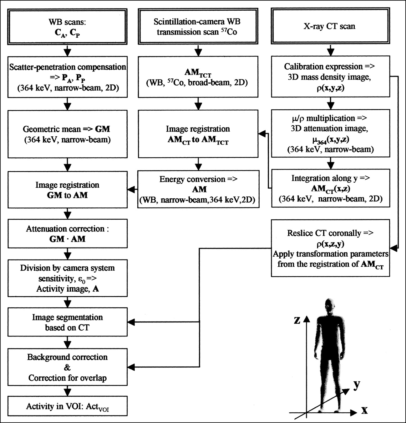
Flow chart of activity quantification method using 3 different image types: anteroposterior WB scans, WB scintillation camera transmission scan, and CT scan. Coordinate system used is shown at bottom. Text in bold denotes images. CA = raw anterior scan; CP = raw posterior scan; PA = primary-count-rate image, anterior; PP = primary-count-rate image, posterior; AMTCT = attenuation map from scintillation camera transmission scan; ρ(x,y,z) = mass density distribution; GM = geometric mean image; AMCT = attenuation map from CT scan; μ/ρ = mass attenuation coefficient; AM = energy-converted WB attenuation map; actVOI = VOI activity.
The WB attenuation map was obtained by combining information from the transmission scan and the CT (Fig. 1). From the 57Co transmission scan, a WB attenuation map, AMTCT, was obtained. From the CT study, a 3D image of the linear attenuation coefficient distribution for 364 keV, μ 364(x,y,z), was determined, which was integrated along the anterior-posterior direction, yielding the attenuation map AMCT. Image registration of AMCT to AMTCT was then performed. The intensity of AMTCT was adjusted according to that of AMCT, yielding the final attenuation map, AM valid for 364 keV.
For image segmentation, the CT image was first resliced coronally, and each coronal slice was then registered to AMTCT (and thus GM) by applying the spatial transformation determined in the registration of AMCT to AMTCT. To avoid time-consuming 3D segmentation, outlining of organs in the full CT set was not performed. Instead, the segmentation was done in 2D by browsing through the coronal CT slices and manually editing a contour until it encompassed the outer limits of the organ, with the intention of determining a maximum area in the x-z plane. The organ thickness, that is, the y-extension, was determined from precalculated organ-background thickness fractions of the total patient thickness. The organ thickness was used in the correction for background activity and overlapping organs.
Imaging Systems
Scintillation camera acquisition was performed on a DIACAM camera (Siemens Gammasonic, Inc., Chicago, IL) connected to a NucLearMAC (Scientific Imaging, Inc., Littleton, CO) computer system. A high-energy parallel-hole collimator was used for 131I measurements and a low-energy, all-purpose collimator was used for 57Co. A 15% energy window, centered at 364 keV for 131I and at 122 keV for 57Co, was used. For the transmission studies, an uncollimated 57Co flood source was mounted on the camera head at a distance of 100 cm, and images were acquired with and without the patient present. WB images, composed of 384 × 1,024 2.4 × 2.4 mm2 pixels, were acquired with a scan speed of either 10 or 20 cm/min.
CT scanning was performed with a Tomoscan LX (Philips Medical Systems, Best, The Netherlands). For all studies, the program for abdominal scanning was used. The transaxial field of view was between 350 and 420 mm, the matrix size was 512 × 512, and axial sampling was performed with a slice thickness of 10 mm and no interslice gaps. A 3D matrix with dimensions of 192 × 192 × 512 and voxel dimensions of 4.8 × 4.8 × 4.8 mm3 was interpolated and then resliced in x-z planes so that a set of coronal CT slices was obtained.
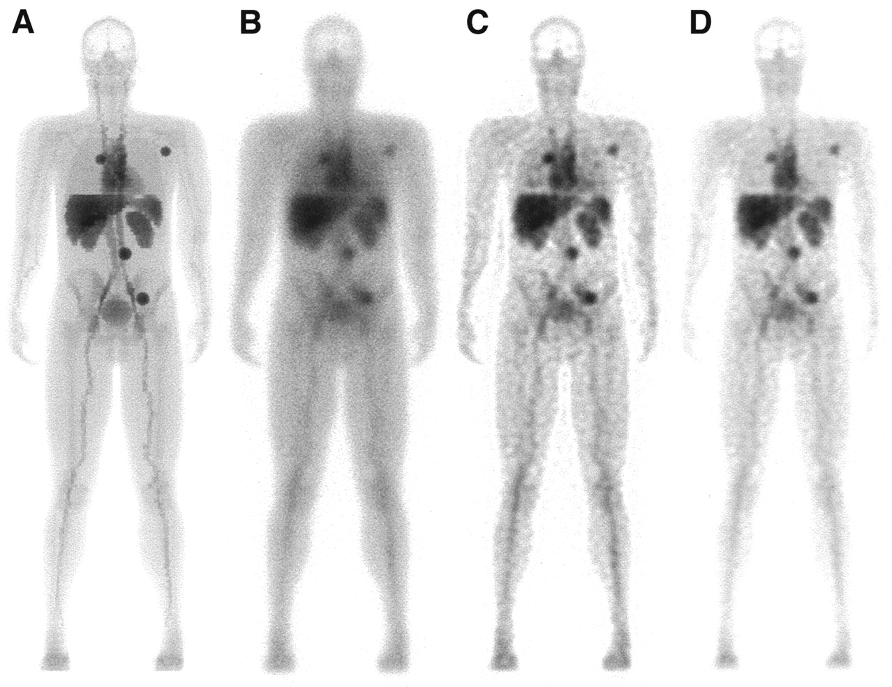
Monte Carlo simulation of 131I emission and 57Co transmission images was performed using a WB anthropomorphic computer phantom (20,21). The SIMIND code was used, together with a routine that allows photon interaction and penetration in the collimator septa (22,23). The activity distribution was defined to resemble that of the RIT studies. Four spherical tumors were defined with diameters of 3.6 or 2.9 cm, situated retriperitoneally, inguinally, at the axilla, and at the right lung hilus (Figs. 2A and B). Transmission studies of 57Co were simulated with and without the phantom interposed. A 3D mass density image was obtained by assigning density values to the various phantom organs (24,25), and this image was used to mimic a CT study.

Simulated images of activity distribution that mimics current patient group. Images were obtained as the geometric mean of anterior and posterior projections. (A) Image representing defined activity distribution, obtained by analytic integration. (B) Monte Carlo simulated image, for the camera system used. (C) Image corrected for scatter and septal penetration. (D) Image corrected for attenuation, scatter, and septal penetration.
Scatter and Septal Penetration Compensation
Compensation for scatter and septal penetration was performed by deconvolution using the following model for image formation (26):
 Eq. 2 where C(x,z) is the measured image; P(x,z) is the projection of the distribution of 131I atoms, which at decay emit 364-keV photons (i.e., the primary count rate distribution); and PRF(x,z) is the point-response function, that is, the planar image obtained in response to a point source in tissue. Deconvolution was performed in frequency space by inverse filtering using a Wiener filter (27–29):
 Eq. 3 where FT denotes the Fourier transformation. The optimal value of the dimensionless parameter K depends on the image signal-to-noise ratio and was applied to achieve a compromise between the noise amplification of the inverse filtering, and scatter and resolution recovery. For this application, the value of K was selected interactively on the basis of the visual appearance of the image.
The applied method was originally developed for 99mTc images (26), on which scattering mainly occurs in the patient. For 131I, the scatter component is more complex because of the high principal energy (364 keV) and the contribution of higher-energy photons (mainly 637 and 723 keV), which, through interactions, may have an energy that makes them detectable within the energy window (3). The PRF used included photons that were scattered in the patient, scattered in the crystal and subsequently escaped, back-scattered in the material behind the crystal, and scattered in or penetrating the collimator septa. These effects were thus compensated for by the deconvolution. Because the PRF is dependent on the source-to-camera distance and the source depth in tissue, 3 different PRFs were included (Fig. 3). All were obtained from Monte Carlo simulation using the SIMIND code (3,22). Simulation of a point source, located centrally in a water-filled phantom with an elliptic cross-section, was performed. The major semiaxis of the ellipse was fixed at 20 cm, whereas the minor semiaxis was varied: 10, 15, and 20 cm for source-to-camera distances of 15, 20, and 25 cm, respectively. For each depth, the volume under the PRF was set to the respective total-to-primary ratio, which was obtained from simulations by recording the primary and the total events separately. The PRFs were angularly averaged to reduce possible artifacts caused by direction-dependent collimator star patterns. When the deconvolution was applied, the PRF that best matched the patient thickness, determined from the attenuation maps, was chosen. As an alternative to performing scatter correction before the formation of the GM image, the GM image was formed from the raw data images and then scatter compensation was applied to it. This was done because the PRF of geometric mean images has been shown to be less depth dependent than the PRFs of separate projections (28,30).
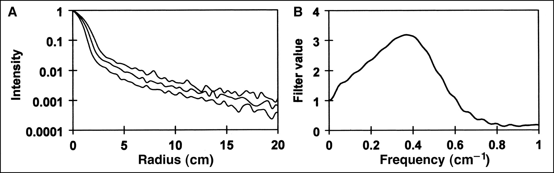
(A) Radial PRFs used for deconvolution scatter and penetration compensation. PRFs for depths of 20, 15, and 10 cm in water, in order from top to bottom. (B) A deconvolution filter that was applied to clinical image in Figure 6, using PRF for a depth of 10 cm.
Attenuation Correction
CT-Based Attenuation Map
CT imaging yields a 3D image of the linear attenuation coefficient of tissue, μhv_CT(x,y,z) (cm−1), for the energy spectrum of the scanner. To apply the CT study for attenuation correction, conversion to 364 keV, μ364(x,y,z), is required. The method presented is based on the observation that for the energy range of interest for RNT (∼140–511 keV), the mass attenuation coefficient,  shows little variation between tissues (24,25). A map of the mass density distribution, ρ(x,y, z), was therefore derived from the CT study, from which the distribution μ 364(x,y,z) was obtained by multiplication by
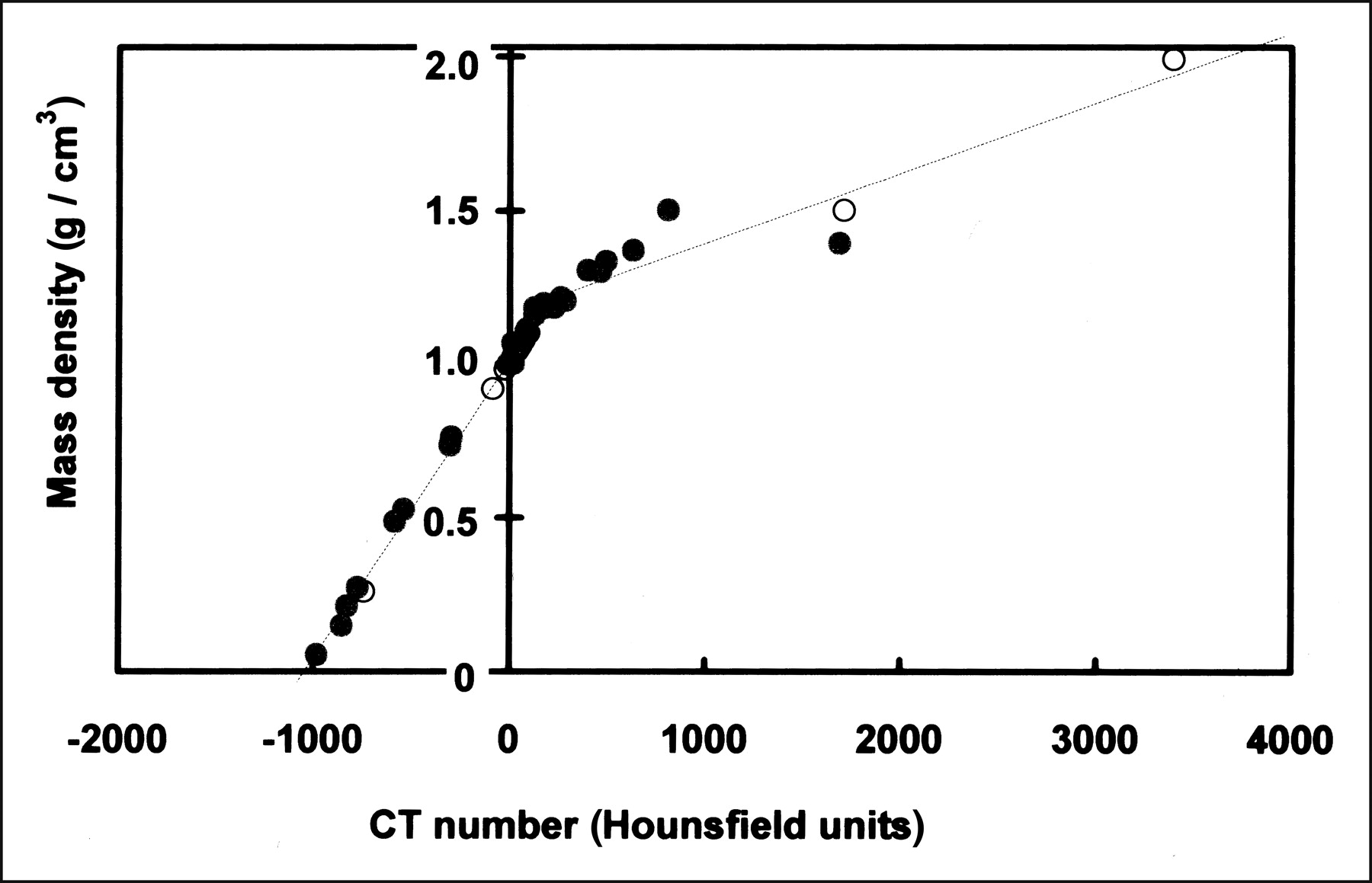
  To determine a relationship between the mass density and the CT number, an experimental measurement of a set of calibration samples was performed (31). The mass density of the samples was determined from calculations based on the electron densities given in Knoos et al. (31) and also by weighing. Furthermore, a set of theoretic CT numbers was calculated for 25 kinds of human tissue (24). These were obtained by summation of the values of μhv_CT, weighted by their relative occurrence according to the spectral distribution of the CT scanner. A bilinear relationship between the mass density and the CT numbers, expressed in Hounsfield units (HU), was established using linear regression (Fig. 4) (31):
 Eq. 4 where H1 is a discriminator value. After calculation of the 3D distribution μ364(x,y,z), a 2D attenuation map, AMCT(x,z), was calculated by line integration along the anterior-posterior direction (Fig. 1):
 Eq. 5 where Δy denotes the pixel dimension in the y-direction (cm). The 2D image NT(x,z) describes the number of pixel sides that represent the patient. It was calculated from the 3D CT study by applying a threshold value that discriminates the patient voxels from the surrounding air (≈ −950 HU), setting all voxels located below the patient couch to a value of zero and then counting the number of voxels that represented the patient in the y-direction for each (x,z).

Calibration of Hounsfield units of CT images to values of mass density. Values were obtained from experimental measurements of set of calibration materials (•), and theoretic values were calculated as sum of linear attenuation coefficient values weighted by spectral distribution of CT scanner (○). Dashed line represents bilinear relationship that was fitted to data.
Scintillation Camera-Based Attenuation Map
From the transmission scan, a WB attenuation map, AMTCT, was obtained:
 Eq. 6 where C(x,z) and C0(x,z) represent transmission count-rate images measured for 57Co with and without the patient in position. Because the measurement is performed in broad-beam geometry, AMTCT describes the effective attenuation, described by μeff,57Co. AMTCT is converted to values of 364 keV in narrow-beam geometry by:
 Eq. 7 where μ364 was set to 0.111 cm−1 (25). The value of μeff,57Co is determined for the individual patient through comparisons with AMCT (Fig. 5). This was achieved using an interactive program that allows for manual adjustment of the value of μeff,57Co until the intensity profiles through AMCT and AMTCT coincide.

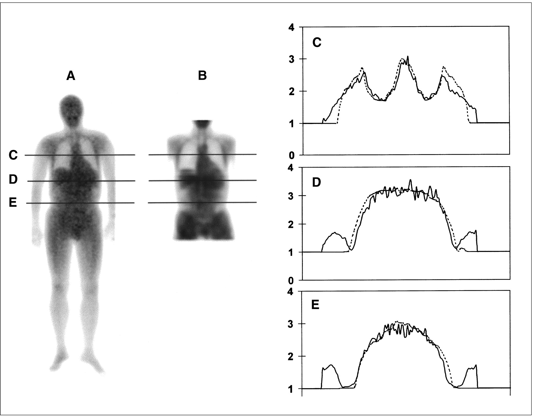
Attenuation maps for 1 patient. (A) The image AM, obtained by energy conversion of attenuation map from WB scintillation camera transmission scanning (AMTCT). (B) Attenuation map obtained from CT (AMCT). (C–E) Plots of attenuation map values, as function of horizontal position, at positions indicated by horizontal lines in images. Profiles of AM (solid line) and AMCT (dashed line).
For the scatter compensation, a value of the patient thickness is required for the selection of the appropriate PRF. The water equivalent thickness was therefore determined as part of the above program, as the water thickness that yields the same attenuation as the maximum value in profiles through AM.
Image Registration
The complete procedure for activity quantification involves 3 instances of image registration (Fig. 1), namely the registration of (a) GM to AM, (b) AMCT to AMTCT, and (c) the coronally sliced CT study to AMTCT (or AM), all of which were accomplished using the registration program described by Sjögreen et al. (20). As AMCT and the coronally sliced CT study arose from the same scan,the registration (c) was performed by direct application of the transformation parameters that resulted from (b) to each slice of the coronally sliced CT, by the assumption that no patient twisting or rolling had occurred. For the registrations (b) and (c) a particular problem was the truncated field of view, and a version of the mutual information criterion that was developed especially for the registration of truncated images (32) was therefore applied.
To interpret the effect caused by imperfect registration on the activity quantification, a separate evaluation was performed using the AM and GM images that were obtained by Monte Carlo simulation, which represent a perfectly matched couple. Random spatial transformations were applied to the AM image, after which registration to the GM image was performed. An activity image was calculated according to Equation 1, and the activity obtained for separate organs was compared with that obtained using the original untransformed images.
Scintillation Camera Sensitivity Calibration
System sensitivity was determined using sources with known activities. Because of the practical difficulties associated with accomplishing a narrow-beam geometry, this measurement was done for sources of varying areas. The assumption was then made that the contribution from scatter and septal penetration increases linearly with the source area and that the contribution can be neglected for an infinitesimal area. Measurements were performed using 3 flat, circular sources (diameters of 57, 33, and 21 mm). The activity of each source was measured in a well chamber (Venstra Instrumenten, Eext, The Netherlands), and imaging was performed at a distance of 10 cm from the camera face. The count density in an ROI placed at the center of each source was measured, and the total number of counts from each source was calculated from the known areas. Division by the activity for each source yielded a sensitivity value, εR, for each area, R. A straight line was fitted to the εR versus R data, the intercept of which on the y-axis gave a value of the sensitivity for R = 0; ε0. This was compared with the sensitivity obtained from Monte Carlo simulation imaging of a point source in air for the same camera system. The number of primary events in this case was registered separately, from which a value of ε0 was calculated.
Correction for Background and Overlapping Organs
Background Correction
The activity of VOIs was determined from the activity image A(x,z) (Eq. 1) using the 2D ROIs that were manually segmented using the coronally sliced CT (Fig. 6), as described earlier in the Materials and Methods. The background subtraction works by determining a background concentration (MBq/voxel) from which the background contribution to the particular ROI is calculated. The ROI volume, VR (voxels), was defined as the volume enclosed by the ROI and the average patient thickness at the ROI location. VR was assumed to contain the VOI and background tissue. The average thickness of the background compartment,  (pixel sides), was calculated from:
 Eq. 8 where
  is the average patient thickness at the ROI location, R is the ROI area (pixels), and NT(x,z) is the thickness distribution of the patient, obtained as described in association to Equation 5. The organ-background thickness fraction, aVOI, is the fraction of the total patient thickness that represents background tissue, which was obtained according to:
 Eq. 9 where
  is the VOI average thickness and VVOI is the VOI volume (voxels). Values of aVOI were calculated in advance and were retrieved at application. For organs, aVOI was calculated using 2 human models, the Zubal anthropomorphic phantom (21) and the analytic MIRD phantom (33) (Table 1). For VOIs other than organs, such as tumors, the value of aVOI was estimated by the operator.

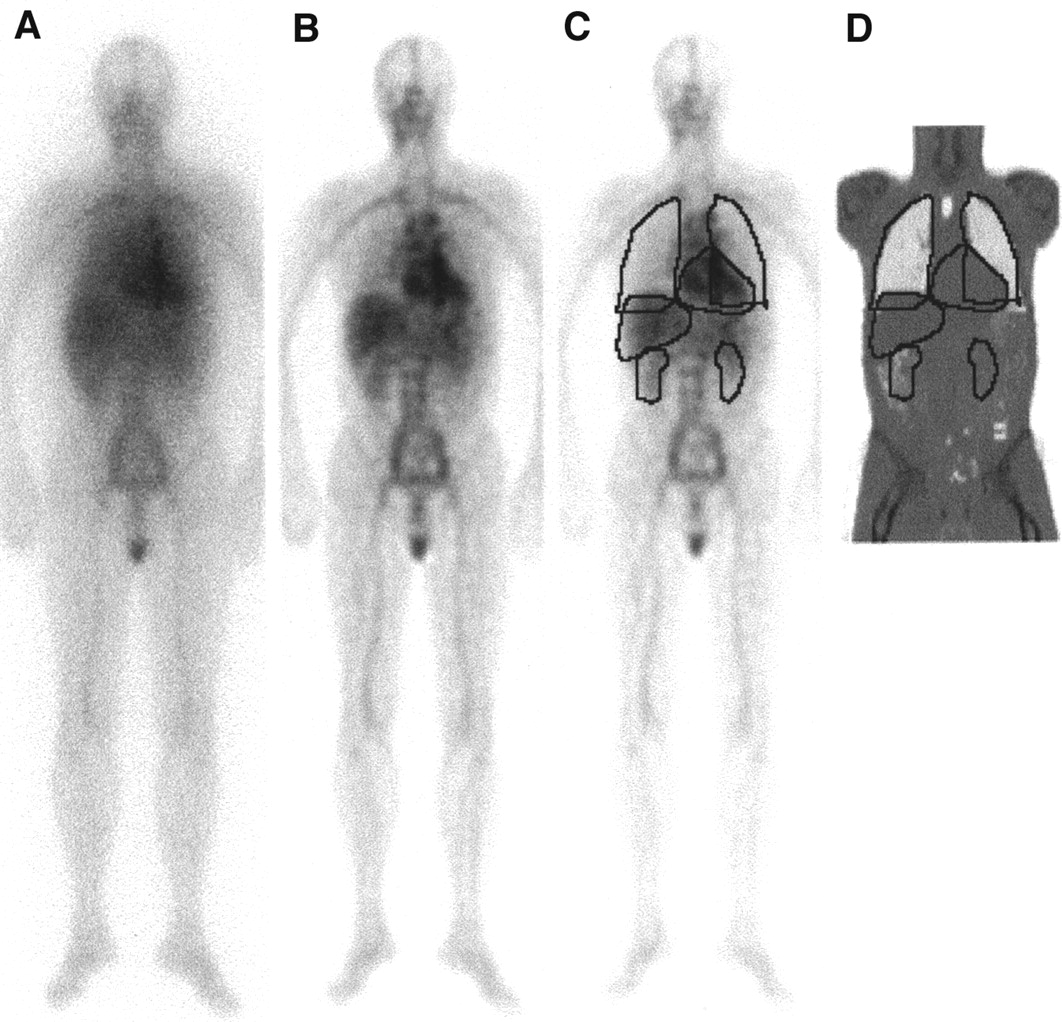
Clinical geometric mean image acquired at 24 h after therapeutic injection. (A) Raw data image. (B) Image corrected for attenuation and scatter penetration. (C) Quantification of organ activities using regions defined from CT, applied to activity image, A(x,z). (D) Coronal CT slice, for which marked regions were manually segmented in slices where outer boundaries of organs were best visualized.
Organ-Background Thickness Fraction, aVOI (Eq. 9), Calculated for Organs from 2 Human Models
The activity in a VOI, ActVOI, was calculated from:
 Eq. 10 where AVOI(x,z) is the background-compensated ROI distribution, AR(x,z) is the distribution within the ROI in the image A(x,z), f corrects for the self-attenuation of the VOI (2) and is calculated for the thickness
  (cm), CBG is the concentration of the background activity (MBq/voxel), and the product
  has the dimensions (MBq/pixel). The value of CBG was determined by measurements in the image A(x,z) in an ROI that contained background only, giving a value ActBG. The volume of this region, VBG, was determined as the sum
  Assuming the background has a uniform concentration throughout the patient, CBG was calculated as the ratio CBG = ActBG/VBG.
Correction for Overlapping Organs
If, in the activity projection image, the VOI was overlapped by other tissues, a separate calculation was performed for the overlapped pixels. The activity distribution AVOI(x,z) was calculated according to Equation 10, but only for the coordinates (x,z), which belonged to the nonoverlapped part of R. For the overlapped pixels, AVOI(x,z) was then determined to the smallest of the following: (a) the average pixel activity of the nonoverlapped pixels; (b) AVOI(x,z) according to Equation 10, ignoring the overlap; or (c) AR(x,z) minus the activity in the overlapping pixel and half the background value, 
For alternative (c) to come into effect, the activity of the overlapping tissue must first be calculated. An organ for which this was applicable for the current patient images is the liver. The activity of the kidneys was first calculated where alternative (a) gave an adequate estimate because of a homogeneous activity distribution. Compensation for the overlap of the right kidney and the liver was then performed using alternative (c).
RESULTS
Scatter and Septal Penetration Compensation
The total-to-primary ratios obtained were 2.44, 2.67, and 2.84 for water depths of 10, 15, and 20 cm, respectively (Fig. 3). A generally improved image quality was obtained because of the resolution and contrast recovery of the deconvolution filter, which is clearly seen in Figures 2 and 6. However, nonhomogeneous activity patterns may result for some structures, for example, the liver and kidneys in Figure 2C.
Attenuation Correction
The constants for the mass density calibration (Eq. 4) were determined to be the following: a = 1.01 g/cm3, b = 9.6 · 10−4 g/cm3/HU, c = 1.12 g/cm3, d = 2.3 · 10−4 g/cm3/HU, and H1 ≈ 200 HU (Fig. 4). An experimental evaluation of the calibration was performed by CT measurement of 2 phantoms, a nonuniform Alderson phantom and an elliptic Jaszczak phantom containing water and a contrast agent. From the Alderson phantom, the following densities were obtained: lungs, 0.3–0.5 g/ cm3; soft tissue, 0.95–1.05 g/cm3; and bone, >1.1 g/cm3. Values given by the manufacturer were as follows: lungs, 0.32 g/cm3; soft tissue, 1.03 g/cm3; and a bone density slightly lower than that of ICRU 46, where it ranges between ∼ 1.2 and 1.9 g/cm3 (25). For the Jaszczak phantom, the densities obtained were as follows: water, 0.95–1.05 g/cm3; acrylic, 1.1–1.25 g/cm3; and the contrast agent, 1.3–1.4 g/cm3. Reference values for water and acrylic are 1.0 and 1.2 g/cm3, respectively (34), and the contrast agent was weighed, giving a value of 1.34 g/cm3.
The Alderson phantom was also imaged by transmission scanning. The 2 attenuation maps, AM and AMCT, were compared by pixel-by-pixel subtraction, from which the average difference was 0.1 ± 0.3. By visual inspection of the difference image, it was seen that the differences were randomly distributed in the abdomen and pelvis, whereas for the thorax, AMCT had somewhat higher values between and at the edges of the lungs. For patient images this tendency was also seen (Fig. 5), and other differences were caused by noise, differences in resolution, misregistration, and the presence of the arms. Furthermore, for the pelvis, AMCT showed a larger variability than AM, with lower values for the projection lines between the pelvic bones and higher values directly above. The values of μeff,57Co obtained were between 0.140 and 0.155 cm−1 for all experiments and patients.
Image Registration
The impact of the registration on the activity quantification was evaluated for the organs listed in Table 2 and the 4 simulated tumors. For 50 independent registrations, the activity obtained was a factor of 0.98–1.01 times the true activity, with a SD of <0.02. The maximum value obtained was 1.07, for the spleen, and the minimum value was 0.94, for the tumor situated at the lung hilus.
Activity Calculation and Its Percentage Error Relative to Known Activity
Scintillation Camera Sensitivity Calibration
The value of ε0 obtained from the extrapolation measurement was 24.3 cps/MBq. The SD was estimated to be 0.5 cps/MBq, based mainly on the uncertainty in the number of counts, particularly for the smallest source, for which resolution effects were not negligible. From the simulation, a value of 24.1 cps/MBq was obtained. Because of the good agreement, the simulated value was considered verified. The sensitivity in scan mode was found to be a factor of 4.9 times less than the sensitivity in static mode. For the activity quantification (Eq. 1), a value of ε0 of 4.9 cps/MBq (=24.1/4.9) was therefore used.
Correction for Background and Overlapping Organs
Validation was performed in analytically generated images of the WB Zubal phantom without the influence of physical factors such as attenuation, scatter, or limited spatial resolution (Fig. 2A). To validate the background compensation, activity was assigned to 1 organ at a time and a homogenous background. Using Equation 10, the activity obtained was a factor of 0.99–1.0 times the true activity. The significance of the background correction was tested for the heart by setting the value of aheart to the values zero and 1 (Eq. 8). A value of zero corresponds to neglecting the background correction, which gave a recovery of 1.42 times the true activity. A value of 1 subtracts a background value that corresponds to the whole patient thickness, which gave a recovery of 0.89. The correction for overlapping organs was evaluated for the activity distribution used in the Monte Carlo simulation. The results varied with the degree of overlap and the amount of activity in the overlapping organ, with obtained recoveries of between 0.94 and 1.06.
Activity Quantification
The activity quantification method was evaluated using the Monte Carlo simulated images and the density image to mimic a CT study. The activity in 6 organs was quantified and compared with the true activity (Table 2). The physical extension of the spleen, liver, kidneys, and lungs was derived from the phantom as the outer boundary of the organs in the projection image. For the heart, the true activity was defined as the sum of the blood and heart wall activity. For the sacrum, the true activity was defined as the blood and bone marrow activity contained within an ROI that was defined manually. The total thickness of the phantom was 20–22 cm at the thickest parts, which corresponds to a water equivalent thickness of up to 24 cm. The results are therefore presented for scatter-penetration compensation using PRFs for depths of both 10 and 15 cm. Results are also presented for quantification using either AM or AMCT for attenuation correction (Table 2). Good results were obtained for all organs included, with deviations of <21%. Using the PRF for 10 cm, the activity of the total image was slightly overestimated, whereas for the 15-cm PRF an underestimate was obtained. This was the case for most organs, although the liver activity was overestimated for both PRFs. Attenuation correction using AM or AMCT generally gave comparable results, with the largest differences being for the heart, lungs, and sacrum. Like the patient images, the AM image had slightly lower values between the lungs and higher values within the lungs. Similarly for the sacrum, the higher resolution of the AMCT image yielded lower values between the pelvic bones, at the sacrum position. In addition to the organs listed in Table 2, quantification was performed for the 4 simulated tumors. Consistent underestimates were here obtained of between −6% and −47%, varying with the tumor location. Given the tumor diameters of only 2–2.5 times the full width at half maximum, the partial-volume effect, and the different background level at the different image locations, the quantification for small volumes was limited.
When the order of the scatter correction and the formation of the geometric mean were reversed, the results were similar to those given in Table 2. Differences of 1%–2% were obtained for most organs, although larger differences (4%–6%) were obtained for the lungs and the sacrum. No tendency could be seen, however.
DISCUSSION
A method for conjugate-view quantification has been presented that uses a CT study in conjunction with WB scans. The method is simple to apply, because most of the procedures included can be performed automatically and are implemented as parts of an interactive program. Monte Carlo simulation has been valuable for evaluation, because the shape and spatial distribution of organs, the overlap in the projection images, and the heterogeneous attenuation and scattering of surrounding tissue can be imitated in a realistic manner.
The scatter-penetration correction was based on isotropic and stationary PRFs, whereas in reality, the scatter component depends on the source depth and the composition of surrounding tissue. Because planar images reflect activity located at various depths, an approximation is introduced when a single PRF is applied for the correction. For the simulation study, the PRF for a depth of 10 cm slightly underestimated the scatter-to-total ratio, whereas for the 15-cm PRF, the ratio was overestimated. The consistent overestimate of the liver activity is believed to be due to boundary effects that were not properly modeled. A large portion of the liver is close to the body boundary, where the scatter distribution changes. The compensation method may be improved using a refined assembly of the PRFs, for example, by interpolation or adjustment to the density of surrounding tissue. In this study, the parameter K was chosen on the basis of the visual appearance of the image. Because the primary objective was to achieve good quantification, and resolution effects are known to decrease the accuracy, comparatively noisy and structured images were preferred over a smooth appearance. Effects such as those seen in Figure 2C, where nonhomogeneous patterns appear, were thus obtained. If the filtering were applied for purposes of image enhancement for diagnostics, another filter setting would be required.
The choice of 57Co for transmission scanning was made because the solid flood-source is easy to handle in clinical practice and the source uniformity is well documented. An energy scaling is required, but this would most likely be required even if using a 131I flood-source, because the objective is to determine an attenuation map for 364-keV photons without the contribution from high-energy photon scattering or septal penetration. A drawback with the scaling is the use of a single parameter (μeff, 57Co) for the entire field of view, because it varies slightly between anatomic regions. Furthermore, the noise level may be significant because of a limited flood-source activity.
For the CT-based attenuation map, the accuracy in the μ-distribution is largely determined by the calibration between mass density and the CT number. For denser materials, a spread in the experimentally measured values was obtained, and the theoretically deduced values were therefore used as a complement. An advantage of using mass density as the calibration quantity is that attenuation maps for any energy used in RNT can be obtained, by multiplication by the appropriate value of μ/ρ. If the CT-based map is to be used directly for attenuation correction, a larger axial span than that available in this study would be required. The limited field of view of the attenuation map restricts the number of organs that can be quantified. Furthermore, we have previously found (20) that the presence of the shoulders and the crotch is critical for the registration between emission and transmission images, and for the current patient studies, the transmission scan was therefore needed as a registration link between the CT and emission images. The differences between the activity distributions obtained when using the attenuation maps from transmission scanning or CT were small; possibly a slight improvement is gained using CT (Table 2).
The consistent underestimate in activity for the 4 simulated tumors is believed to be due to partial-volume effects combined with a limited image contrast. The limited spatial resolution in scintillation camera imaging imposes both a spill-out from the source to the background and a spill-in from the background into the source (35). For small volumes, the quantification is thus less accurate, and further method development is required in this area.
From the analytic simulation results, it was concluded that the value of the organ-background thickness fraction aVOI is not critical, and values based on phantom geometries (Table 1) yield sufficient results. Overlap of organs is deemed to be the largest source of uncertainty, because the compensation relies on a subjective choice of the order in which the organs are quantified.
An advantage of the presented quantification method is that each physical effect is corrected for separately, which makes it straightforward to extend to other applications. To be used for another radionuclide, only 3 parts need to be modified: the value of the camera system sensitivity, the assembly of PRFs, and the value of μ/ρ obtained from reference data for the generation of the CT-based attenuation map.
CONCLUSION
The method presented for activity quantification in different organs was able to quantify the activity distribution to within 10%. Scatter-penetration compensation by deconvolution gave acceptable accuracy for most organs, although the assembly of PRFs may be refined for situations in which they deviate from an isotropic estimate. CT was found useful for the segmentation of organs and for background compensation. Currently, both CT and scintillation camera transmission scanning are used for attenuation correction. When CT scanning with a large axial field-of-view is enabled, it will be of interest to apply the CT-based attenuation map directly for attenuation correction. Future development will also involve an investigation of the background-dependent partial-volume effect, for an improvement of the quantification of small activity volumes.
Acknowledgments
The authors thank Dr. Jan Boucek of the Fremantle Hospital, Western Australia, for implementation of the voxel-based MIRD phantom. The authors would also like to thank Stefan Johnsson, MSc, and Tommy Knoos, PhD, Department of Radiation Physics, Lund University Hospital, for providing the CT calibration material and measurements. Thanks are also due to Ola Lindén, MD, Department of Oncology, Lund University Hospital, for rewarding discussions. This study was funded by the Swedish Cancer Foundation, the Gunnar Nilsson Foundation, the Berta Kamprad Foundation, the Royal Physiographic Society, the John and Augusta Persson Foundation, and the Lund University Hospital Foundations.
Footnotes
Received Sept. 10, 2001; revision accepted Mar. 25, 2002.
For correspondence or reprints contact: Katarina Sjögreen, PhD, Department of Radiation Physics, Lund University Hospital, SE-22185 Lund, Sweden.
E-mail: katarina.sjogreen{at}radfys.lu.se
REFERENCES
In this issue


Jump to section
Related Articles
Cited By...
- Dosimetric Quantities in Neuroendocrine Tumors over Treatment Cycles with 177Lu-DOTATATE
- Long-Term Retention of 177Lu/177mLu-DOTATATE in Patients Investigated by {gamma}-Spectrometry and {gamma}-Camera Imaging
- 90Y Bremsstrahlung Imaging for Absorbed-Dose Assessment in High-Dose Radioimmunotherapy
- Uncertainties in Internal Dose Calculations for Radiopharmaceuticals
- Toward Patient-Friendly Cell-Level Dosimetry
- A 3-Dimensional Absorbed Dose Calculation Method Based on Quantitative SPECT for Radionuclide Therapy: Evaluation for 131I Using Monte Carlo Simulation