


Abstract
Active bone marrow is one of the more radiosensitive tissues in the human body and, hence, it is important to predict and possibly avoid myelotoxicity in radionuclide therapies. The MIRD schema currently used to calculate marrow dose generally requires knowledge of the patient's total skeletal active marrow mass—a value that, at present, cannot be directly measured. Conceptually, the active marrow mass in a given skeletal region may be obtained given knowledge of the trabecular spongiosa volume (SV) of the bone site. A recent study has established a multiple regression model to easily calculate total skeletal SV (or TSSV) based on simple skeletal measurements obtained from a pelvic CT scan or radiograph. This model, based on data from only 20 cadavers, did not account for sex differences in TSSV. This study thus extends this work toward sex-specific models. Methods: Twenty male and 20 female cadavers were subjected to whole-body CT. Bone sites containing active bone marrow were manually segmented to obtain SV at each site. In addition to age and height, 14 CT-based skeletal measurements were recorded for each cadaver. Multiple linear regression techniques were used to determine the best subset of measurements that allowed an accurate prediction of TSSV. Results: A pooled model (R2 = 0.76) and a sex-specific model (R2 = 0.79) are provided. A leave-one-out analysis reveals that these models predict total SV with less than 10% error for 50%–70% of subjects, and with less than 20% error for 70%–90% of subjects. Tables were constructed that provide the percent distribution of SV in active-marrow containing bone sites for both males and females. Conclusion: This study provides models that can be used to simply, yet accurately, predict total SV in individuals within the clinical setting. The models require only 2 or 3 skeletal measurements that can be easily measured on a pelvic CT scan. Even though this study does not conclusively determine which model is best at predicting TSSV, the sex-specific model is most consistent at providing reasonable estimates of TSSV. This study also explains how the predictive TSSV model can be used to estimate patient-specific active bone marrow mass under the assumption of reference values of marrow volume fraction and bone marrow cellularity by skeletal site.
- bone marrow
- radionuclide therapy
- spongiosa volume
- active bone marrow mass
- radiation dosimetry, patient-specific, sex-specific, male, female
A primary goal in molecular radiotherapy is to optimize various treatment parameters—radionuclide, carrier molecule (peptide, antibody, pharmaceutical), administered activity, use of pretherapy drugs (cold antibody, amino acids, etc.)—to maximize tumor cell kill while minimizing toxicity in nontargeted tissues. The dose-limiting toxicity most frequently encountered in molecular radiotherapy is myelosuppression for protocols that do not provide a priori for stem cell support (1). Accurate and patient-specific assessments of the radiation-absorbed dose to the hematopoietically active (or red) marrow (AM) in patients under clinical trials are thus essential to the establishment of dose–response relationships needed for prediction of these effects in future cancer patients (2,3).
For radiopharmaceuticals that bind to marrow tissues or to mineral bone, explicit knowledge of the patient's total and, in some cases, regional active marrow mass is required for proper scaling of radionuclide S values (4), which are in turn assessed in a reference computational phantom or skeletal model (5,6). Under the assumption that no adjustments are required of the radiation-absorbed fraction—fraction of emitted particle energy that is absorbed in the target tissue—patient-specific S values to AM from radiopharmaceuticals localized in skeletal source tissue rS may be estimated as: Eq. 1where mAM is the total active marrow mass in either the reference phantom or the patient. Although values of mAM may be taken from the radiation protection literature for reference patients, it remains a significant challenge to measure or even estimate values of mAM in a live patient of vastly different or even similar body morphometry. Values of mAM for a reference 35-y male and female are given in ICRP Publications 70 and 89 as 1,170 g and 900 g, respectively (7,8).
Conceptually, the value of (mAM)patient may be calculated using the following expression: Eq. 2where SVx is the volume of trabecular spongiosa, MVFx is the marrow volume fraction, and CFx is the marrow cellularity factor, all assessed at skeletal site x, with ρAM being the mass density of active bone marrow (1.03 g cm−3 as given in ICRU Report 46 (9)). “Spongiosa” refers to the combined tissues of the bone trabeculae and marrow (active and inactive) within cancellous bone and is, therefore, exclusive of cortical bone at the cortex at each skeletal site. The “marrow volume fraction” (MVF) is that fraction of spongiosa volume occupied by marrow tissues (i.e., not occupied by the bone trabeculae). “Marrow cellularity” is then the fraction of marrow tissue volume that is hematopoietically active and, for marrow tissues with normal extracellular fluid volumes, it may be considered approximately equal to (1 − fat fraction). The skeletal regions to consider in the adult for Equation 2 (variable x) would be those of the axial skeleton as well as the proximal epiphyses of the humeri and femora (7). As shown in the second formulation of Equation 2, values of SVx in a skeletal site x can alternatively be represented as the product of the total skeletal spongiosa volume (TSSV) and its fractional distribution by skeletal site x (
 ). Neither of these variables is defined in reference patients used in nuclear medicine dosimetry (7,8).
To apply Equation 2 for a given patient, one must assess, bone-by-bone, values of SV, MVF, and CF—obviously an impractical and, in the case of MVF, virtually impossible task. Magnetic resonance techniques do exist, however, to noninvasively measure CF, but these techniques have been applied only selectively in larger skeletal regions (e.g., pelvis, lumbar vertebrae) (10,11). In lieu of clinically feasible methods of assessing patient-specific values of MVF and CF, clinicians may continue to rely on data acquired for purposes of radiological protection. In ICRP Publication 70 (7), literature values of both bone volume fraction (BVF = 1 − MVF) and marrow cellularity are given in Tables 15 (page 27) and 41 (page 68), respectively. Although these are not officially “reference” values, they may be provisionally adopted as such in the application of Equation 2 to patient-specific estimates of mAM. These values are given in Table 1 of this study, along with reference values for the percentage mass distribution of active bone marrow in the adult. As will be noted, the coefficients of variation of  given in the present study are noted to be very small and, thus, can be applied with confidence in current patient studies.
Percentage Distribution of Active Bone Marrow, Bone Volume Fractions, and Marrow Cellularity Within Adult Skeleton (41–50 y) as Given in ICRP Publication 70 (7)
Values of MVF are both age- and sex-dependent owing to natural processes of mineral bone loss with age and the fact that osteopenia and osteoporosis are typically accelerated in older females. Mean cadaver-based estimates of BVF are given in Table 15 of ICRP 70 (7) in decade increments for adults 21–30 y to 81–90 y for the vertebrae and iliac crest, whereas additional values of BVF are given for the femur, ribs, and parietal bone for only the age range 41–50 y. Due to limited sample sizes, data for males and females are combined. Values of CF in Table 41 of ICRP 70 (7) give only a single set by bone site for the 40-y adult and, thus, are not given as a function of age or sex. Meunier et al. (12), however, indicate that as bone trabeculae thin, the additional marrow space is primarily occupied by adipocytes and, thus, the age-dependent product of MVF and CF might possibly remain constant with age in normal marrow. Consequently, the data in Table 1 may perhaps be used in Equation 2 irrespective of patient age.
The most important determinant of mAM in Equation 2 is the patient-specific estimate of TSSV. To address this clinical need, Brindle et al. (13,14) developed a predictive equation for patient-specific TSSV requiring only 2 measurements in a pelvic CT—os coxae width (OC.W) and os coxae height (OC.H). Their predictive equation is: Eq. 3Equation 3 was constructed using multiple linear regression on data from 20 cadavers—10 males and 10 females. SV was determined from manual segmentation of full-body CT images. A leave-one-out analysis showed that the above equation is able to make TSSV predictions with errors that range from 0.2% to 21.2%, with most errors being under 11% (15).
Because of limitations in sample size (due in part to the tedious nature of the data collection), the predictive model of Equation 3 was based on pooled data from both sexes. However, male and female skeletal dimensions are expected to be different. In fact, these differences are used by forensic scientists to ascertain the sex of a crime victim given access to skeletal remains. Males are usually larger than females in both height and weight (16,17). As a consequence of differences in biomechanical loading experienced in weight-bearing bones, femur length and femoral head diameter are greater in men than in women (18,19). Vertebral width is also found to be greater in males (17). Furthermore, it is known that several pelvic dimensions are larger in females than males, and although the differences in anatomy may be related to the fact that females give birth, nonreproductive factors may also be at play (18).
The objective of the present study was to expand the study of Brindle et al. (14) to construct sex-specific predictive models of TSSV, along with sex-specific estimates of its fractional distribution within the skeleton for clinical applications of Equations 1 and 2. Given that the human skeleton is subject to sexual dimorphism, one would expect that a predictive model that includes a sex-discriminating variable will be more effective at predicting TSSV than a model that does not make this distinction.
MATERIALS AND METHODS
The methods used in this article are similar to those described previously in Brindle et al. (14) and, hence, are only briefly outlined here. When a method differs significantly from that in our earlier study, a more detailed description is given.
Cadaver Selection
In our previous study, whole-body CT images from 20 cadavers (10 male and 10 female) were acquired for the purpose of determining SV by skeletal site. In the present study, we have extended the data pool to 40 cadavers through the acquisition of an additional 10 males and 10 females. As before, all cadavers were acquired via approved procedures from the State of Florida Anatomic Board. The targeted age range was 40−80 y as representative of cancer patients potentially treated with radionuclide therapy. Each candidate was screened and excluded if the cause of death or previous medical condition was indicative of excessive bone loss. Finally, a body mass index (BMI) of between 18.5 and 24.9 kg m−2 was additionally targeted as representative of average nonobese adults (20). Though ethnicity was not a selection factor, all cadavers selected for this study were white.
Image Acquisition
Each cadaver was imaged on a Siemens Sensation 16 CT scanner in the Department of Radiology of Shands Hospital at the University of Florida. The slice thickness for each was 2 mm with an in-plane resolution of 977 μm. The scan spanned from the top of the head to slightly above the middle of the femoral shaft. Given that it is difficult to discern the location of trabecular spongiosa in the skull at full-body scan resolution, the head of each cadaver was imaged separately at a slice thickness of 1 mm and an in-plane resolution of approximately 450 μm.
SV Estimation
SV was obtained by manual segmentation using an IDL-based code (Interactive Data Language; IDL version 6.0; ITT Visual Information Solutions, Inc.) written by our group (21). The bone sites segmented were those identified by the International Commission on Radiological Protection (ICRP) Publication 70 (7) as those containing hematopoietically active bone in the adult. SV for the mandible and cranium where obtained from the separate head scans. The sites and their reported percent contribution of active bone marrow are given in Table 1 as recommended in ICRP Publications 70 (7) and 89 (8).
Given the significant time (approximately 1 mo per cadaver) and effort required of the manual segmentation process, 8 individuals (referred to as “segmenters”) were used in the segmentation of the 20 additional cadaver scans. To ensure consistency and quality in the segmentation effort, all segmenters underwent identical training, developed and administered by the first author of this article. All segmentation files were visually inspected by the first author for quality assurance purposes. The accuracy of the manual segmentation and the magnitude of intersegmenter variability have both been investigated by Brindle et al. (15).
Anatomic Measurements
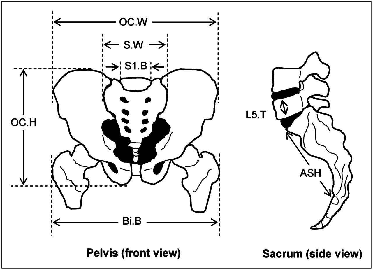
The rationale for our choice of anatomic measurements is outlined in Brindle et al. (13). Measurements have been focused primarily on the os coxae primarily because (i) a large percentage of the TSSV is located in this site (7,14,22) and (ii) measurements can be easily performed on a pelvic CT. These measurements may also be made from the CT portion of a SPECT/CT or PET/CT sessions used to quantify skeletal uptake of the radiopharmaceutical (4). The skeletal measurements considered in this study are summarized in supplemental Table S1 (supplemental Tables S1–S4 are available online only at http://jnm.snmjournals.org). Graphical representations of these measurements are given in Figures 1 and 2.

Graphical representation of pelvic measurements described in Table 2. OC.W = os coxae width; S.W = sacral width; S1.B = S1 breadth; OC.H = os coxae height; Bi.B = bitrochanteric breadth; L5.T = L5 thickness; ASH = anterior sacral height (supplemental Table S1).
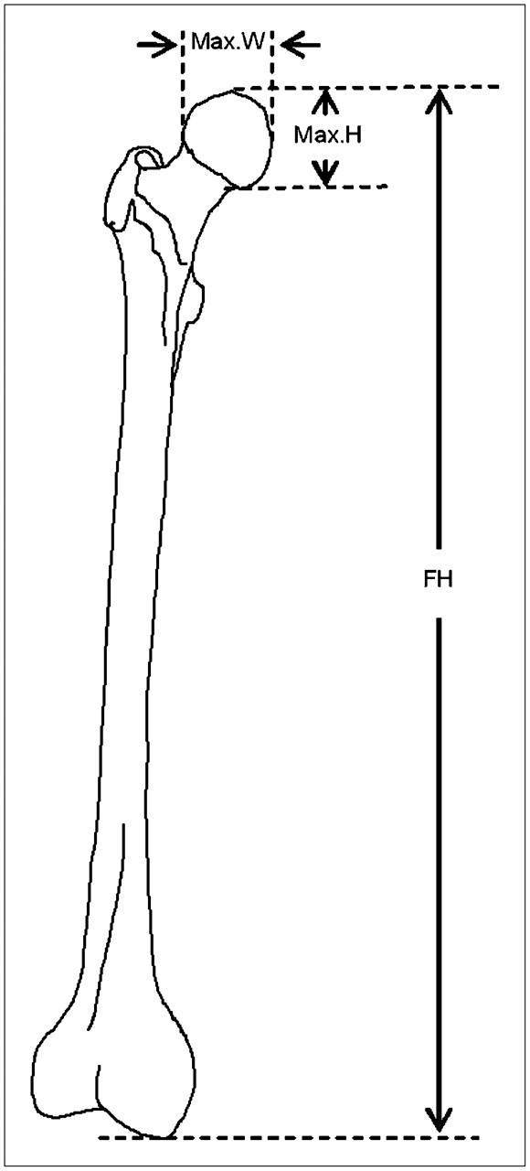
Graphical representation of femoral measurements described in Table 2. Max.W = maximum width of femoral head; Max.H = maximum height of femoral head; FH = femoral height (supplemental Table S1).
Many of the skeletal measurements described in supplemental Table S1 are based on the methodology of Moore-Jansen et al. (23). With the exception of body height and femoral height, all measurements were made using the plug-in Volume Viewer v.1.21 (24) of the software ImageJ v.1.36b (25). Body height and femoral height were measured using DicomWorks v.1.3.5 (26) on the anterior–posterior scout images produced during CT image acquisition. Given that no CT scout image spanned the entire length of a study cadaver, total body height was calculated as the sum of 2 measurements: the vertical distance from the top of the head to the top of a proximal femoral head, and the vertical distance from the top of the same femoral head to the bottom of the heel on the same leg.
Volume Viewer allows the user to rotate the CT image in 3 dimensions (3D). This feature is useful as cadaver positioning cannot be changed (i.e., rigor mortis) and in many cases the pelvis was not parallel to the CT table. If one measures, for example, the width of the pelvic bone using the scout image, the measurement may be underestimated due to the tilt of the pelvis. By being able to rotate the CT image in 3D, one can take a snapshot of the pelvis when it is “parallel” to the screen and, hence, make a more accurate measurement. Even though Volume Viewer allows the user to view the pelvis in 3D, measurements are actually made on snapshots taken from the 3D rendering and are, therefore, 2-dimensional.
All measurements were performed in duplicate. Measurements were made over the span of several weeks and, hence, are not sequential. The delay between corresponding duplicates was sporadic and of sufficient length so that the likelihood of bias from prior measurement recall was minimal.
Statistical Analysis
All statistical calculations required for the construction of the predictive equations were made using the statistical software JMP IN version 5.0 (SAS Institute Inc.). Multiple linear regression analysis was used to select an optimal set of predictor variables (from supplemental Table S1) that could be used to predict TSSV. The general equation for the regression model is: Eq. 4where
  is the intercept,
  are the coefficients for each of the predictor variables
  , and
, and  is the error associated with the model.
There are many criteria that can be used to determine the subset of independent variables that best fits the data. In general, it is a good idea to use more than one criterion, because if different criteria result in the selection of the same subset of variables, this can be taken as confirmation that the optimum subset has been selected (27). The same criteria used in Brindle et al. (14) were applied in the selection of the best subset of variables in the present study: (i) stepwise selection, (ii) adjustedR2, (iii) Aikake Information Criterion (AIC), and (iv) Bayes Information Criterion (BIC).
The AIC is a leading criterion in model selection (28,29), the objective being to select a subset of variables that minimizes the value of AIC. However, if the sample size is small one should instead use the corrected AIC (AICc) (28–30). Accordingly, the AICc was used in this study in lieu of AIC.
The model-building process was started by producing models that did not include a sex variable—these models are referred to as “pooled”. The first step is to examine all possible models that can be constructed using subgroups of the 15 predictor variables. The JMP software produces a table that lists all possible models composed of all 15 variables, subsets of 14, and so on, all the way down to 1-variable models. This results in thousands of possible models. JMP automatically calculates R2 and adjusted R2 for each model. AICc and BIC values were calculated by means of a script. A plot of each criterion statistic versus the number of variables was used to determine the optimal model for each criterion.
The sex-specific model was constructed following the procedure just described, with the difference that a dummy variable for sex was added to the set of predictor variables. The variable was defined as: Eq. 5This is the preferable way to introduce sex specificity into a model, rather than constructing separate models for each sex, because the regression includes the entire dataset and, hence, all measurements contribute to estimation of the regression parameters (27). In addition, the coefficient that multiplies the dummy variable may provide insights into differences between male and female subjects (31).
RESULTS
The cadaver dataset used in this study is shown in supplemental Table S2 and is inclusive of data from the Brindle et al. study (14). Values of active marrow mass given in the final column of supplemental Table S2 are estimates using Equation 2 and data from Table 1. Supplemental Table S3 allows us to compare our skeletal measurements with similar measurements found in the literature for white males and females in the United States (19,32–34). We were unable to find values in the literature for some of our skeletal dimensions—for example, Bi.B, OC.H—and, hence, they are omitted from the table. Values of TSSV were also omitted from the table because, to our knowledge, SV has not been measured by any other research group. Supplemental Table S3 includes skeletal measurements obtained from The Forensic Data Bank (FDB) accessible via the software FORDISC 2.0 (34). The FDB contains skeletal data for about 1,400 individuals from the United States, which include both sexes and different ethnicities. Data from the Hamann-Todd collection (3,000 skeletons held at the Cleveland Museum of Natural History) are accessible via the Web site http://www.cmnh.org/site.
Supplemental Table S4 shows the predictor variables selected using each criterion and the resulting R2 and adjusted-R2 values for the model. Two categories of models are shown: “pooled” models, based on all data and do not discriminate sex; and “sex-specific” models, based on all data and discriminate sex by means of a dummy variable (Eq. 5). Models that included too many variables to be of practical use, variables with large P values (>0.3), or variables that were highly collinear, were not considered for further analysis. These models have been marked with an asterisk and the reason for rejection is stated in the final column.
A leave-one-out analysis was produced to estimate the accuracy of prediction for each model. Percent error was calculated from the difference between the predicted and measured TSSV values. Figure 3 provides percent error histograms for each model listed in supplemental Table S4.
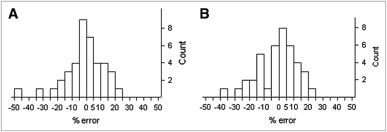
Percent error histograms. (A) Pooled model. (B) Sex-specific.
Table 2 provides the coefficients and relevant statistics for each of the predictor variables included in the models recommended for clinical use in this study. The models were selected based on the following criteria: (i) smaller number of variables, (ii) higher R2 value, and (iii) model selection criterion used. Given that AICc has been shown to be superior over other model-selection criteria (30), models selected by this criterion were preferred.
Parameters for Recommended TSSV Predictive Models
DISCUSSION
Our skeletal measurements are consistent with the expected ranges for white North Americans (supplemental Table S3). In spite of our small sample size for each sex (n = 20), our mean skeletal measurements are very close to those calculated from much larger sample sizes.
Supplemental Table S4 provides the models selected by the different criteria. In the case of pooled models (i.e., no sex discrimination), all criteria except for adjusted R2 agree on a 3-variable model that includes OC.H, Bi.B, and P. The model selected by the adjusted-R2 method was rejected because it contains 2 variables—P and FD—that are highly collinear and because the coefficients for FD and L5.T have large P values—0.24 and 0.17, respectively.
Figure 3A shows the percent error histogram for the pooled model calculated from the leave-one-out analysis. The highest prediction errors are obtained for cadaver 26 (45.4% error) and cadaver 29 (31.2% error). “Studentized” residuals identify both of these cadavers as moderate outliers (2.5 ≥ |t| ≥ 2.0) in our cadaver dataset. These cadavers are also extremes in our cadaver dataset, representing unusually large or unusually small values for the predictor variables, or for TSSV. Given that the model tries to fit to the data used to create it, one can expect to find larger errors in individuals that present skeletal dimensions or TSSV that are uncommon.
The sex-specific models were constructed with the addition of a dummy variable for sex, as defined in Equation 5. The model chosen by the stepwise-mixed method was rejected on the basis that P and FD are highly collinear and have coefficients with large P values: 0.22 and 0.36, respectively. The model selected by AICc was chosen over the other 2 models, first, because it was selected by AICc and therefore given greater weight, and, second, because it is simpler, only requiring 2 skeletal measurements.
Figure 3B presents the percent error histogram for the sex-specific model. Cadaver 31 shows the worst prediction with an error of −35.2%. Even though this cadaver is not an extreme in our cadaver set, it presents very small values for OC.H, Bi.B, and TSSV, and it is an extreme in the male cadaver set, with the smallest values in TSSV and OC.H in males. Cadavers 26 and 29, previously identified as extreme in the discussion of the pooled model are predicted with −22.8% and −25.4% error, respectively.
The final models recommended by the authors are provided in Table 2. Table 3 shows the percentage of cadavers that were predicted best by each of the recommended models on the basis of the absolute magnitude of the percent error of prediction. Both models fair equally well in the prediction of TSSV in females, but the sex-specific model is superior at providing good predictions for males. Table 4 shows the percentage of cadaver TSSV predictions that have absolute errors less than or equal to 5%, 10%, 15%, and 20%. The differences in performance between the models for male and female TSSV prediction are, at worst, 15% (3 of 20 cadavers), whereas differences in overall performance are, at worst, 7% (3 of 40 cadavers).
Percentage of Cadavers for Which Each Model Was Best at Predicting TSSV as Determined by Absolute Value of Percent Error of the Prediction
Percentage of Cadaver TSSV Predictions that Had Absolute Errors Less than or Equal to 5%, 10%, 15%, and 20%
Even though Tables 3 and 4 do not conclusively show which type of model should be used to predict TSSV in males and females, the authors lean toward the sex-specific model for 3 reasons. First, the sex-specific model is better at accurately predicting TSSV in males and is slightly better at predicting TSSV in both sexes (Table 3). Second, it does a better job at predicting TSSV in individuals that are unusual and, therefore, difficult to predict. Cadavers 26 and 29 are extremes in our cadaver dataset. The sex-specific model predicts these 2 cadavers with smaller errors than the pooled model, with cadaver 26 resulting in an error of −25.75% versus −45.42% and with cadaver 29 resulting in an error of −25.43% versus −31.21%. Third, the sex-specific model accounts for sex differences in skeletal morphology. Several skeletal dimensions are different in males and females. t tests on the data of supplemental Table S2 reveal that, at least for the individuals in our study, males are larger in height, os coxae height, S1 breadth, femoral head perimeter, Feret's diameter, maximum height and width of the femoral head, humeral height, and femoral height (all tests with P value < 0.0005). t tests also reveal that values of SV are larger (P value < 0.005) in males in all bone sites measured with the exception of the cranium and mandible. TSSV is also larger in males (P value < 10−7). These differences in SV may be a consequence of the fact that males are generally larger than females. However, when we grouped the SV data into equal height ranges, we found a large spread in SV values in each height group, thus suggesting that the difference in the distribution of SV in adult males and females may not be due to differences in height. We do not have enough cadavers to perform good statistics when the cadavers are grouped by height and even less so when we then separate by sex; hence, we can only provide insights into the sexual dimorphism of the skeleton and SV distribution of males and females.
Our models are unintentionally based on cadavers belonging to individuals of one racial group—white. It is well known that skeletal dimensions exhibit differences related to race and geographic location (16,19,35–37). Accordingly, caution must be used when using our models to predict TSSV in patients of other races.
In Table 5, we give values of  —the fractional distribution of TSSV by skeletal site. Two sex-averaged sets of
  are given—one from the study of Brindle et al. (14) on 20 cadavers, and one from the current study on 40 cadavers (inclusive of the former). Mean values of
  are essentially unchanged, with the additional data only evident in changes to the SD. Table 5 also provides values of
  for males and females. Two-tailed t tests show that the fractional distribution of TSSV is significantly different in males and females in the cranium (P < 0.0001), the mandible (P = 0.0054), the scapulae (P < 0.0001), the ribs (P = 0.0022), the sacrum (P < 0.0001), and the proximal humeri (P < 0.0001).
Percent Regional Distribution of Trabecular Spongiosa by Skeletal Site in Bones Known to Contain Active Marrow in Adult
Values of  in Table 5 may be used for 2 clinical purposes. First, they may be used along with predictive TSSV models in the evaluation of Equation 2. In the assumption that values of BVF and CF in Table 1 are appropriate for a given patient (i.e., in lieu of patient-specific data), Equation 2 can be evaluated for either the adult male or adult female patient as:
 Eq. 6
Eq. 6 Eq. 7where the TSSV multiplier differs only with respect to differential sex changes in
  . Clearly, more information is needed on both the age and sex dependences of BVF and CF as well as patient-specific methods for their measurement. For example, cadaveric values of BVF may be acquired via bone harvesting and micro-CT analysis and then empirically tied to individual patients through quantitative CT-based assessments of volumetric bone mineral density in the lumbar vertebrae (measurements that can be performed on both the patient of interest and the cadaver of the source tissues). Similarly, MRI or MR proton spectroscopy volunteer studies can be conducted to further parameterize (by age, sex, disease state, prior chemotherapy, etc.) the very limited age- and sex-averaged values of marrow cellularity given in ICRP Publication 70 (7).
Second, image-based methods of radiopharmaceutical activity concentration in the skeletal tissues are usually performed on selected regions of interest (ROIs) such as the sacrum, femoral head, or portions of the lumbar vertebrae. Once a regional estimate of marrow (or bone) activity is made via PET or SPECT, this activity may be proportionally scaled to yield a total skeletal estimate of radiopharmaceutical marrow or bone activity. Values of  in Table 5 can be used for just this purpose. For lumbar vertebrae imaging, the ROI is typically restricted to L2–L4 due to the need to avoid ROI overlap with the pelvis or urinary bladder. As shown at the bottom of Table 6, these 3 vertebrae account for, on average, 6.08% and 6.16% of TSSV (corresponding to ∼8.6% and ∼8.9% of active marrow mass; Table 6) in the adult male or females of our 40-subject study, respectively. Within the sacrum, some 6.8% and 8.1% of TSSV (corresponding to ∼9.6% and ∼11.6% of active marrow mass; Table 6) is found in male and female patients, respectively. Caution must be exercised, however, in the use of
  for regional scaling of marrow activity when the radiopharmaceutical skeletal uptake is not uniform across all skeletal sites.
Percent Regional Distribution of Active Bone Marrow Mass by Skeletal Site
The data of Tables 1 and 5 may be used in combination with Equation 2 to establish values of the percent mass distribution of active bone marrow  in both sexes:
 Eq. 8
Eq. 8
As the patient-specific value of TSSV from the predictive regression equations cancels in Equation 3, these male and female values of  are not patient-specific per se but are more akin to reference values as based on mean values of
  in this study. Values of
  from Equation 3 are shown in Table 6, where sex differences stem only from changes in
  and not from changes in MVF and CF (as only sex-averaged mean values are given in ICRP 70 (7)). These estimates may then be compared with the sex-averaged reference values given in ICRP Publication 70. Discrepancies between the ICRP 70 model and the sex-dependent distributions of this study (values greater than 2%) are noted for the cranium, lumbar vertebrae, and os coxae in the male model and for the cranium, ribs, and lumbar vertebrae in the female model. While the male and female distribution data shown in Table 6 from this study are based on image-based measurements of SV, the ICRP 70 (7) reference distribution of mAM comes from an analysis by Cristy (38) using data originally published by Mechanick (39). The cadavers of this 1926 study were victims of prolonged wasting illnesses, which rendered them relatively emaciated and which might have led to significant changes in the tissue components (22). As noted by this author, the process by which Mechanick measured marrow mass was not clearly explained in his original paper (22). Of particular note is the overly large assignment of active bone marrow to the cranium (7.6%), a value that is not supported by the range of SV obtained in this current 40-subject study (percent mAM of 2.7% in males and 4.3% in females). Nevertheless, it is cautioned that the male and female distributional values in Table 6 may be further improved after the creation of more patient-specific methods of assigning both MVF and CF in the evaluation of Equation 2 for individual patients.
CONCLUSION
In this study, pooled and sex-specific models are presented (Table 2) that can be used to predict total skeletal spongiosa volume in a given patient with an error generally expected to be within ±10%–20% (Fig. 3; Table 4). The models require values of only 2 or 3 skeletal dimensions that are easily measured on pelvic CT images. The study does not conclusively determine which type of model—pooled versus sex-specific—is best at predicting TSSV. However, the authors favor the use of the sex-specific model as it generally provides the best predictions (Table 3), is more accurate in predicting TSSV in patients of atypical skeletal morphometry, and accounts for sex differences. In situations where it is necessary to know SV at a particular bone site, values of percent volume distribution of SV among bone sites are given (Table 5). The predictive equation provides patient-specific TSSV, and the product of TSSV and the percent distribution of SV by bone site yields the SV (in cm3) for the bone site of interest. Clearly, direct CT volumetry in the skeletal site of interest would yield a more accurate result. In addition, it is noted that patients of unusually small or large skeletal stature will be poorly predicted by the models of Table 2. Under the further assumption of “reference” values for both marrow volume fraction and marrow cellularity by skeletal site, the patient-specific estimate of TSSV can be used in Equations 6 and 7 to yield an estimate of total active bone marrow mass within individual male or female patients, respectively. Further research is required, however, in the development of clinically feasible methods of assessing these histologic parameters on an individual basis, thus further improving the patient specificity of method presented here.
Acknowledgments
The authors thank the following individuals for their assistance in performing the manual image segmentation portions of the study (alphabetical by last name): Ryan DuBose, Daniel Hendrick, Dr. Derek Jokisch, Alexa Kapilow, Paul Moore, Dominic Pare, Dr. Phillip Patton, Thomas Roomy, Jessica Salazar, and Lindsay Sinclair. This study was supported by Grants RO1 CA96441 and F31 CA97522 from the National Cancer Institute with the University of Florida.
Footnotes
-
COPYRIGHT © 2007 by the Society of Nuclear Medicine, Inc.
References
- Received for publication June 20, 2007.
- Accepted for publication August 8, 2007.


Jump to section
Related Articles
Cited By...
- Skeletal energy homeostasis: a paradigm of endocrine discovery
- Biodistribution, Tumor Detection, and Radiation Dosimetry of 18F-DCFBC, a Low-Molecular-Weight Inhibitor of Prostate-Specific Membrane Antigen, in Patients with Metastatic Prostate Cancer
- MRI Measurement of Bone Marrow Cellularity for Radiation Dosimetry