


Abstract
The current gold standard for measuring marrow cellularity is the bone marrow (BM) biopsy of the iliac crest. This measure is not predictive of total marrow cellularity, because the biopsy volume is typically small and fat fraction varies across the skeleton. MRI and localized MR spectroscopy have been demonstrated as noninvasive means for measuring BM cellularity in patients. The accuracy of these methods has been well established in phantom studies and in the determination of in vivo hepatic fat fractions but not for in vivo measurement of BM cellularity. Methods: Spoiled gradient-echo in vivo images of the femur, humerus, upper spine, and lower spine were acquired for 2 dogs using a clinical 3-T MRI scanner. Single-peak iterative decomposition of water and fat with echo asymmetry and least squares (SP-IDEAL) was used to derive BM fat fractions. Stimulated-echo acquisition mode spectra were acquired in order to perform multipeak IDEAL with precalibration (MP-IDEAL). In vivo accuracy was validated by comparison with histology measurements. Histologic fat fractions were derived from adipocyte segmentation. Results: Bland–Altman plots demonstrated excellent agreement between SP-IDEAL and histology, with a mean difference of −0.52% cellularity and most differences within ±2% cellularity, but agreement between MP-IDEAL and histology was not as good (mean difference, −7% cellularity, and differences between 5% and −20%). Conclusion: Adipocyte segmentation of histology slides provides a measure of volumetric fat fraction (i.e., adipocyte volume fraction [AVF]) and not chemical fat fraction, because fat fraction measured from histology is invariant to the relative abundances of lipid chemical species. In contrast, MP-IDEAL provides a measure of chemical fat fraction, thus explaining the poor agreement of this method with histology. SP-IDEAL measures the relative abundance of methylene lipids, and this measure is shown to be equivalent to AVF. AVF provides the appropriate parameter to account for patient-specific cellularity in BM mass predictive equations and is consistent with current micro-CT–based models of skeletal dosimetry.
- IDEAL
- fat–water separation
- bone marrow
- cellularity
- radioimmunotherapy
- adipocyte volume fraction
- fat fraction
Radiation-induced bone marrow (BM) toxicity occurs as a result of damage to hematopoietically active marrow (AM), and hence accurate and patient-specific assessments of the radiation-absorbed dose to the AM in patients under clinical trials are essential to the establishment of dose–response relationships needed to predict these effects in future patients (1–2). AM absorbed dose is typically estimated using the MIRD schema (3):
This mass of AM in a given patient may be estimated, however, using the expression:
Direct measurement of the parameters TSSV and
In cell biology, marrow cellularity is measured as the volume fraction of marrow occupied by hematopoietic stem and progenitor cells. However, in radiation dosimetry, CF is generally interpreted as the volume fraction of marrow not occupied by adipocytes. This definition, in part, stems from the construction of computational models of skeletal dosimetry in which, at their finest level, voxels of BM are tagged as either hematopoietically active or inactive marrow, with the latter defined as the marrow adipocytes (9–10). The voxel size applied in these micro-CT–based models is either 30 or 60 μm, the latter corresponding to the average diameter of adipocytes in human BM (11).
The parameter CF, as defined for the purpose of radiation dosimetry, is a quantity that can be determined noninvasively in a patient. If we assume that the fat content of hematopoietic cells is negligible in comparison to that of adipocytes, and that the water content of adipocytes is negligible compared with that of the remainder of soft-marrow tissues, CF is also equivalent to 1 minus the volume fat fraction. Both MRI and proton magnetic resonance spectroscopy (H-MRS) have been used to measure fat fractions in BM (12–13) and liver (14–17). Hence, it is possible to measure CF noninvasively in a patient using MRI or H-MRS.
In this study, fat fractions by bone site are determined by fat–water separation through the iterative decomposition of water and fat with echo asymmetry and least squares (IDEAL) method (18). Most fat–water separation methods estimate fat fractions by considering only the signal of the majority lipid, methylene (CH2), inevitably resulting in an underestimation of true fat fraction. IDEAL can be performed with consideration of multiple lipid resonances, thus accounting for a larger fraction of the total fat signal (19). In this study, when IDEAL is based on a single lipid resonance, we refer to it as single-peak IDEAL (SP-IDEAL), and when it is based on multiple lipid resonances, it is referred to as multipeak IDEAL (MP-IDEAL). Even though the in vivo accuracy of IDEAL in the estimation of fat fractions has been adequately characterized for the measurement of hepatic fat fractions (16–17,20), the in vivo accuracy of the technique for BM has not as yet been determined.
MATERIALS AND METHODS
Animal Care and Procedures
The study was conducted with approval from the Institutional Animal Care and Use Committee. Two mongrels (male; age, 1.5 y; weight, ∼25 kg) were purchased from an authorized provider. The University of Florida Animal Care Services provided housing and care for the dogs, transportation, preparation before MRI scans (intubation, anesthesia), monitoring of vital signals, and euthanasia before necropsy, following protocols approved by the Institutional Animal Care and Use Committee.
MRI and Postprocessing
Scans were acquired using a 3-T Achieva MRI scanner (Philips) with a 6-element torso phased-array coil. The anatomy of interest was aligned with or near the center of the coil to obtain approximately uniform sensitivity across the target bone. Dogs were placed in right or left lateral decubitus, feet first. Breath-hold was not used, under the assumption that breathing motion would not be an issue when imaging the upper and lower third of the spine. The long bone that was imaged was pinned between the table and the dog's body and was therefore not expected to move during image acquisition.
Multiecho spoiled gradient-recalled (SPGR) imaging was performed at 2 flip angles—5° and 34°—and 6 echoes were acquired with a first echo time (TE1) of 5.95 ms, ΔTE of 0.38 ms, and repetition time (TR) of 40 ms. Image resolution was maintained at or below 1.0 mm, and chemical shift misregistration was below 1 pixel (the receiver bandwidth varied from 428 to 434 Hz/pixel). Each image acquisition required approximately 30–55 s. The raw image data were saved for each acquisition.
Coronal slices, 7 mm thick, were acquired as parallel to the central axis of the bone as possible. Given that both the spine and the long bones are slightly curved, 2 or 3 slices were acquired to ensure adequate coverage. The following bones were imaged: humerus, femur, upper spine (C4–T3), and lower spine (T10–C7). Slice localization and placement was performed using 3-dimensional SPGR scans of the upper and lower third sections of the body of the dog. Imaging parameters were a TR of 18.3 ms, TE of 1.93 ms, flip angle of 20°, 2 signal averages, and sensitivity encoding factor of 4.0. Each 3-dimensional SPGR localization scan took approximately 10–16 min. MRI sessions lasted for approximately 4 h for each dog.
A MATLAB (The MathWorks) code was written to read and process the raw image data files. The code also reconstructed the complex images from the k-space data extracted from the raw data files and calculated the composite image from the individual coil images using a spatial-matched filter as described in Walsh et al. (21). The noise covariance matrix was assumed to be the identity matrix, and coil sensitivities were estimated from the coil images following the procedure of Erdogmus et al. (22).
Both SP-IDEAL and MP-IDEAL with precalibration were performed on the 6 echoes following the methodology of Yu et al. (19) and the graph-cut algorithm by Hernando et al. (23). Fat–water separation was performed using a MATLAB code provided by Diego Hernando (University of Wisconsin–Madison). The spectra used in the precalibration of MP-IDEAL were derived for each bone site using stimulated-echo acquisition mode (STEAM) as described subsequently. Lipid spectral amplitudes were normalized before implementation into MP-IDEAL. T1 correction of the water and fat images was performed using the methodology described by Liu et al. (24). T2* corrections were not possible, given the short interecho spacing used in the acquisition of the images. T2* for fat and water in human BM at 3 T has been reported in the lumbar vertebra as 73 and 40 ms, respectively (25). Assuming that similar relaxation parameters apply in dog BM, even for the largest TE used (7.9 ms), the T2* decays in water and fat are comparable, so the error in the calculated fat fraction due to T2* relaxation is expected to be negligible.
Regions of interest (ROIs) were defined at the locations for which bone cubes were extracted during necropsy. The location and size of the cubes excised from the long bones were determined from digital photographs taken during necropsy. The digital necropsy photos were calibrated for distance with ImageJ (http://rsbweb.nih.gov/ij/index.html) using the ruler included in each photograph. Once the image was calibrated, distances on the bone with respect to one end could be determined. These measurements were used to place the ROI in the calculated water and fat images at the approximate location from which the bone cubes were extracted for histology, to ensure that CF was measured at the same region on the bone. Because the resolution of the MR images is known, the process to convert distances in pixels to distances in centimeters and vice versa was straightforward. Vertebrae can be accurately identified in the MR images based on physical appearance, and so no distance measurements were required.
CF at each ROI was determined from the calculated water and fat magnitude images as the sum of the pixel intensities inside the ROI in the water image divided by the sum of the pixel intensities inside the ROI in the water and fat images. CF can also be calculated as the average CF value inside the ROI, but it was found that this calculation results in highly unstable estimates.
MR Spectroscopy
Single-voxel spectroscopy was performed using STEAM at selected volumes of interest (VOIs) placed at the head, neck, and shaft of the long bones and in the body of selected cervical, thoracic, and lumbar vertebrae. In the case of the femoral and humeral heads, the VOI was made as large as possible inside the head without including cortical bone or adjacent bone (e.g., scapula, pelvis). VOIs in the necks and shafts of the long bones were adjusted to the thickness or diameter of the bone, but the length was fixed at 1.5 cm to mimic the size of the bone cube to be excised. The VOI in the vertebral bodies was made as large as possible inside the vertebral body without inclusion of the cortical shell. VOIs varied from 1.5 to 7.5 cm. Acquisition parameters were as follows: number of excitations, 16; TR, 2,000 ms; points, 1,024; and bandwidth, 2,000 Hz. TE was set to minimum, resulting in TEs ranging from 9.2 to 13.6 ms. Water peak line widths after shimming ranged from 4 to 8 Hz.
Spectral analysis and fitting were performed using jMRUI (version 4.0) (26) with AMARES (27). Spectra were manually phase-corrected. The expected resonances of the lipid peaks (Table 1) were determined from published human BM spectra (28–31). Soft constraints of ± 0.05 ppm were imposed around the resonances to allow some flexibility to the fitting algorithm. Amplitudes were forced to be real. The selection of line shape (Lorentzian or gaussian) was based on the observed shape of the spectral peaks and the understanding that the presence of trabecular bone will result in line shapes that are typically broadened. Hence, gaussian line shapes were typically selected. Spectral amplitudes in jMRUI correspond to twice the area under the peak.
Lipid Peak Spectral Shifts
A single MR image may include multiple vertebrae or a complete long bone, and MP-IDEAL with precalibration is based on a single spectrum. Hence, for the long bones, a common lipid spectrum was derived by averaging the lipid peak amplitudes from the spectra of the head, neck, and shaft. For the spine, a common lipid spectrum was derived by averaging the lipid peak amplitudes for separate vertebra in each section of the spine. The resulting lipid spectra were normalized before use in MP-IDEAL.
Necropsy and Histology Slide Preparation
Immediately after euthanasia, the dog cadavers were transported to the Small Animal Hospital of the University of Florida, where necropsy was performed to extract bone cubes. Bone cubes were then extracted from the head, neck, and shaft of the long bones. Digital photos were taken of each long bone, including a 15-cm ruler for scale, to show the location of the cuts. One end of the bone was always visible in the photos to allow a reference point from which to measure. The bodies of 2 cervical vertebrae (chosen from C4 to C7), 2 thoracic vertebra (T12 and 1 chosen from T1 to T4), and 2 lumbar vertebrae (chosen from L5 to L7) were also extracted.
Cortical bone and excess soft tissue were removed from each bone cube using a band saw. Finished bone cubes were immediately placed in separate labeled jars containing 10% neutral-buffered formalin in a ratio of bone to fluid by volume of 1:10. Bone cubes with thickness greater than 5 mm were cut in half to ensure that the fixation agent would be able to penetrate the bone completely. Fixation took place for 32–36 h. Once completed, the bone cubes were decalcified by submersion in DecalStat (3% HCl; Decal Co.) for 2–3 h. The University of Florida Molecular Pathology Lab mounted the BM samples on paraffin blocks and produced microscope slides. Each slide consisted of a 5-μm section. For most blocks, a section was obtained from 4 different levels spaced by 200–500 μm, depending on the size of the block. The sections were placed on microscope slides and stained with hematoxylin and eosin using standard protocols.
Histology Slide Sampling
The University of Florida Molecular Pathology Lab scanned each histology slide at high resolution using a slide scanner (Aperio). The Aperio software allows visualization of the entire slide and the selection of rectangular ROIs that can be saved as separate images. Square ROIs with a side of 500 μm were placed inside viable marrow cavities in such a manner that they did not include trabecular bone or regions of missing soft tissue. The size (500 μm) was determined empirically as the largest square side that adequately fits inside most marrow cavities and therefore allows acceptable sampling coverage. ROI images were extracted and saved to separate files that were numbered sequentially. Adequate sampling of each histology slide was determined by plotting the cumulative mean CF after the evaluation of each ROI. Additional ROIs were randomly selected and processed until the plot converged to a steady-state value—that is, when fluctuations in the cumulative mean CF were less than ±1%. A 95% confidence interval was also calculated for each slide to determine that most of the measurements were within this interval. The final step in the study was to determine marrow cellularity in various ROIs within the histologic slides via automated methods of adipocyte segmentation. Details and validation of the method used are given in the Supplemental Appendix (supplemental materials are available online only at http://jnm.snmjournals.org). A graphical description of the process is provided in Supplemental Figure 1, with validation results further provided in Supplemental Figure 2.
RESULTS
MR Spectroscopy
MRI spectra are summarized in Table 2. In jMRUI, the spectral amplitudes correspond to twice the area under the peak and hence the normalized amplitudes represent the fractional abundance of each lipid species. The lipid resonance with a shift of −2.0 ppm (Table 1) was not found in any of the spectra and is therefore omitted from Table 2.
Normalized Lipid Spectra for Each Skeletal Region
IDEAL Fat–Water Separation
Figure 1 and Supplemental Figures 3, 4, and 5 present some of the results of SP-IDEAL fat–water separation performed on the images acquired in the femur, humerus, upper spine, and lower spine, respectively, of the dogs. In most cases, the fat–water separation appears accurate and images seem free of fat–water switches. The regions inside bone are typically noisier than the surrounding soft tissues. This is more clearly appreciated in the field map images (Fig. 1C).

SP-IDEAL water–fat separation in femur of dog. SP-IDEAL was performed on 6 SPGR echoes acquired with flip angle of 5°, TR of 40 ms, TE1 of 5.95 ms, and ΔTE of 0.38 ms. (A) Water image. (B) Fat image. (C) Field map. (D) Composite image (sum of water and fat images).
The long bone that is pinned between the body of the dog and the table was not expected to experience any motion. Figure 1 and Supplemental Figure 3 do not show artifacts from breathing motion near the long bones, but Supplemental Figure 4 does show motion artifacts in the area of the rib cage. In the case of the upper spine, the motion artifacts are clearly observed in the thoracic and abdominal cavities, but these artifacts are not perceptible in the upper vertebrae. The white arrows in Supplemental Figure 4 point to locations where fat–water switches have occurred. These regions have an intensity different from the surrounding areas in the field map image (Supplemental Fig. 3C). In contrast, the images for the lower spine (Supplemental Fig. 5) do not show obvious motion artifacts.
As expected, the fat and water images derived from images acquired with a low flip angle (Fig. 1 and Supplemental Fig. 4) have lower signal-to-noise ratios than those derived from images acquired with a larger flip angle (Supplemental Figs. 3 and 5). However, image quality is quite good, even in the low-flip-angle images.
During necropsy, photos were taken of the long bones cut in half along their main axis. The photographed bone was the contralateral bone that was imaged during MRI. Figure 2 shows the necropsy photograph and the SP-IDEAL–calculated fat image for the femur in 1 of the dogs. Even though there is no reason to expect that fat distributions are the same on the right and left femur (Figs. 2A and 2B), the calculated fat image matches closely the fat distribution in the photo. The match is particularly clear at the distal end of the femur, at which the fat distribution tapers. Excellent matching is also observed in the humerus (Figs. 2C and 2D). The red marrow region that separates the fat at the humeral head from the fat in the shaft matches the dark pattern in the fat image.

Comparison of fat distribution visually observed in long bones with fat distribution in fat images. (A) Necropsy photo of cut across midline of left femur. (B) SP-IDEAL fat image of right femur. (C) Necropsy photo of cut across midline of humerus. (D) SP-IDEAL fat image of right humerus. Fat images were cropped and rotated to match orientation of bone on necropsy photo.
The images resulting from MP-IDEAL with precalibration using the normalized lipid spectra in Table 2 are not shown, because they are visually indistinguishable from those in Figure 1 and Supplemental Figures 3–5. However, the pixel intensities in the fat images resulting from MP-IDEAL were much larger than those in SP-IDEAL, differing by factors as large as 2.0.
Agreement Between IDEAL and Histology
Table 3 summarizes the CF values measured with histology, SP-IDEAL, and MP-IDEAL. Figure 3A presents the linear regression plot of CF measured with SP-IDEAL versus CF measured from histology performed at the same location in bone. Excellent agreement was demonstrated by a slope close to unity (0.98), small intercept (0.83% cellularity), and correlation R2 of 0.98. Figure 3B presents the Bland–Altman plot produced with the same data. Bias is small (less than −1% cellularity), with all differences within 4% and −5% cellularity and most differences within ±2% cellularity. One outlier is identified, corresponding to a measurement performed in L4 in one of the dogs.
BM CF Data

Agreement of CF measured by SP-IDEAL and histology at same location on bone in two dogs. (A) Linear regression fit. (B) Bland–Altman plot. Middle horizontal line corresponds to mean difference, equal to −0.5% cellularity, and top and bottom horizontal lines correspond to 95% confidence interval, equal to 4% and −5% cellularity, respectively. Plot identifies outlier, corresponding to measurement in L4 in one of the dogs.
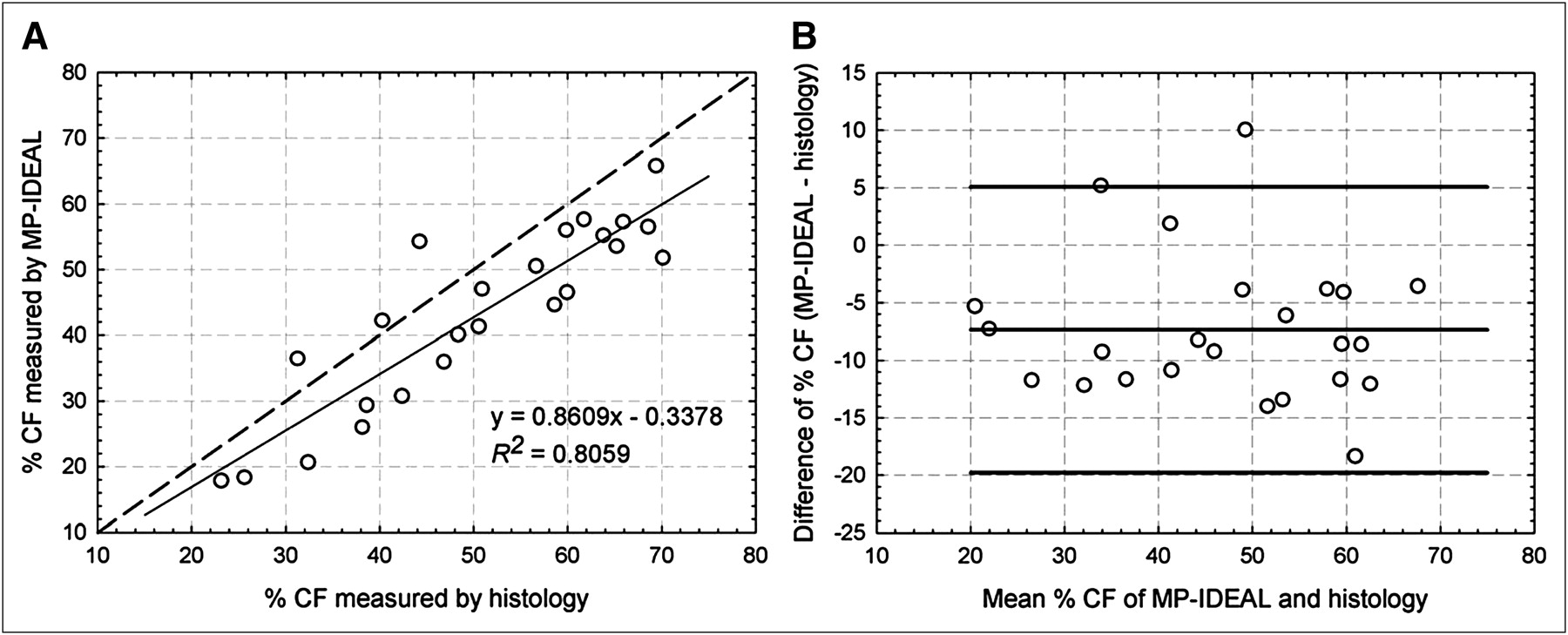
Figure 4A presents the linear regression for the results obtained with MP-IDEAL. In this case, the agreement is not as good as in the case of SP-IDEAL, as demonstrated by a slope of 0.86 and R2 of 0.81. The Bland–Altman plot (Fig. 4B) demonstrates a bias of −7%, with all differences being within 5% and −20% cellularity, except for 1 outlier. The outlier corresponds to the measurement made in C6 in one of the dogs.

Agreement of CF measured by MP-IDEAL and histology at same location on bone in two dogs. (A) Linear regression fit. Dashed line is perfect agreement line. (B) Bland–Altman plot. Middle horizontal line corresponds to mean difference, equal to −7% cellularity, and top and bottom horizontal lines correspond to 95% confidence interval, equal to 5% to −20% cellularity, respectively. Plot identifies outlier, corresponding to measurement in cervical vertebra C6 in one of the dogs.
DISCUSSION
The excellent agreement shown in Figure 3 between SP-IDEAL and histology is not surprising, because the spectroscopy results suggest that the abundance of methylene (CH2) was relatively uniform in all bones of this study. However, considering that methylene accounts only for approximately 75% of lipid content, the closeness of the agreement is quite surprising. The adipocyte segmentation method, as performed in this study, inevitably underestimates fat content, because adipocyte fragments smaller than a preselected diameter are assigned to water. SP-IDEAL also underestimates the fat fraction, because it only accounts for fat originating from methylene molecules. According to Figure 3B, histology CF is typically larger than SP-IDEAL CF (the bias is negative). Since SP-IDEAL measurements are already overestimations of bone marrow CF, histology is also suggested to overestimate bone marrow CF. Hence, the close agreement is most likely a consequence of the underestimation of fat fraction by adipocyte segmentation.
Given that histology is the current gold standard for in vivo CF determination, the close agreement between both methods indicates that SP-IDEAL can be used in lieu of histology. SP-IDEAL is noninvasive and can be performed at any bone on the body, whereas in vivo histology can be performed only at the iliac crest. In addition, because SP-IDEAL provides fat and water images of the complete bone, CF changes can be assessed at multiple locations. These results also indicate that CF measured by SP-IDEAL is sufficiently accurate to be used in BM mass predictive equations (5). A CF error within ±4% will result in a negligible loss of accuracy in most cases.
An advantage of using SP-IDEAL versus MP-IDEAL is that SP-IDEAL does not require the acquisition and analysis of MRS data. However, MP-IDEAL is expected to provide a more accurate measurement of chemical fat fraction because it takes into account multiple lipid resonances. Figure 4A presents the linear regression for MP-IDEAL, and Figure 4B provides the associated Bland–Altman plot. Unexpectedly, the agreement is not as good as that of SP-IDEAL, with MP-IDEAL underestimating CF in most measurements (the bias is −7% cellularity), meaning that MP-IDEAL is consistently measuring a larger fat fraction than histology. All differences, except for an outlier, are within 5% and −20% cellularity.
The disagreement is not an indication of failure by MP-IDEAL. The close agreement between SP-IDEAL and histology demonstrates that histology overestimates CF. Adipocyte segmentation of histology images will yield the same fat fraction regardless of the relative lipid abundances in the adipocytes. However, the fat fraction derived from MP-IDEAL will always be larger than that derived from SP-IDEAL, because the latter accounts only for one lipid species. The Bland–Altman plot (Fig. 4B) shows that almost all MP-IDEAL CF measurements are smaller than those derived from histology. On the basis of the previous calculation of the error in the calculated CF when only 76% of fat is considered, and assuming no error in the determination of water content, the ability of MP-IDEAL to detect higher lipid fractions in adipocytes explains some of the disagreement, approximately 4% cellularity at low and high CF and increasing to 7% cellularity as CF approaches 50%. Figure 4A shows that most differences are smaller than −15%.
CONCLUSION
Our MRS data indicate that although the relative abundance of methylene lipids is fairly uniform throughout the canine skeleton (coefficient of variation, 10%), the relative abundances of the remainder lipid species are highly variable (coefficient of variation, >50%). Adipocyte segmentation of histology images of BM provides a measure of a volumetric fat fraction (i.e., AVF), but it is not a measure of chemical fat fraction, because it is invariant to the relative abundances of lipid species. SP-IDEAL accounts only for methylene lipids, which in the canine skeleton correspond to approximately 75% of lipid content. As such, SP-IDEAL will always underestimate the chemical fat fraction. However, the close agreement shown in Figure 3 indicates that SP-IDEAL based on the methylene resonance provides a measure of AVF as determined with the current gold standard, BM histology. The excellent agreement between the methods indicates that SP-IDEAL can be used to derive the AVF data necessary for the estimation of patient-specific active BM mass using published predictive equations (5).
DISCLOSURE STATEMENT
The costs of publication of this article were defrayed in part by the payment of page charges. Therefore, and solely to indicate this fact, this article is hereby marked “advertisement” in accordance with 18 USC section 1734.
Acknowledgments
We thank Diego Hernando (Department of Radiology, University of Wisconsin–Madison) for providing technical support and MATLAB code for IDEAL fat–water separation using graph cuts. This study was partially funded by the National Research Service Award fellowship F31 CA134200 and grant R01 CA96441 awarded by the National Cancer Institute. No other potential conflict of interest relevant to this article was reported.
Footnotes
Published online Jul. 28, 2011.
- © 2011 by Society of Nuclear Medicine
REFERENCES
- Received for publication January 13, 2011.
- Accepted for publication May 6, 2011.


