


Article Figures & Data
Figures
- FIGURE 1.
Principle of tomographic acquisition and geometric considerations. At each angle, data are projection of radioactivity distribution onto detector. Note that location of any scintillation onto crystal allows one to find out direction of incident photon (dashed line) but not to know distance between detector and emission site of photon.
- FIGURE 2.
(Left) Shepp–Logan phantom slice (256 × 256 pixels). (Right) Corresponding sinogram, with 256 pixels per row and 256 angles equally spaced between 0° and 359°. Each row of sinogram is projection of slice at given angular position of detector.
- FIGURE 3.
(Left) Principle of projection for one 3 × 3 slice at angle θ = 0 and θ = 90°. Value in each bin is sum of values of pixels that project onto that bin. (Right) Example: g1 = f3 + f6 + f9 = 2 + 2 + 3 = 7. Result of projection is sinogram with 2 rows, whose values are (7, 9, 7) and (6, 9, 8).
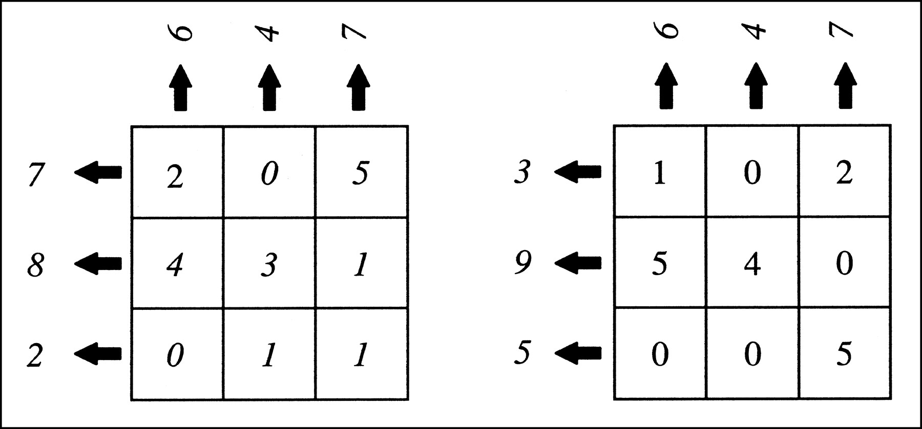
- FIGURE 4.
(Left) Principle of backprojection for one 2 × 3 sinogram. Value in each pixel is sum of values of bins that, given angle of detector, can receive photons from that pixel and is divided by number of rows of sinogram. (Right) Example: f1 = (g3 + g4)/2 = (7 + 6)/2 = 6.5. Compare this slice with that of Figure 3, and note that after 1 projection and 1 backprojection, initial slice is not retrieved.
- FIGURE 5.
Example of 2 distinct images that can yield same projection at angle 0. This illustrates the fact that when number of projections is insufficient, solution (i.e., slice that yields projections) may be not unique.
- FIGURE 6.
Illustration of star (or streak) artifact. (A) Slice used to create projections. (B–G) 1, 3, 4, 16, 32, and 64 projections equally distributed over 360° are used to reconstruct slice using backprojection algorithm. Activity in reconstructed image is not located exclusively in original source location, but part of it is also present along each line of backprojection. As number of projections increases, star artifact decreases.
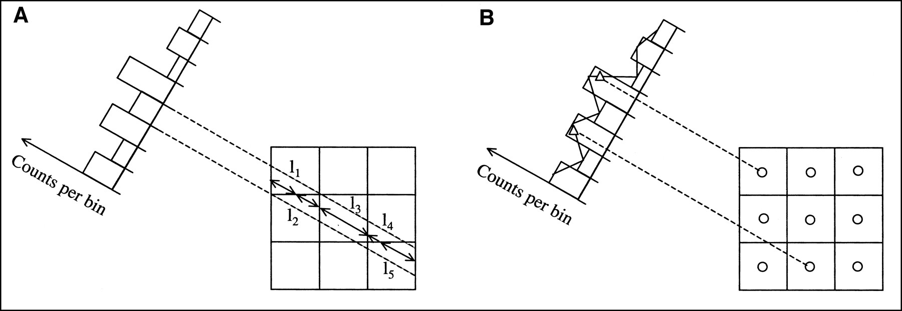
- FIGURE 7.
Modelization of geometry of backprojection. (A) With ray-driven backprojection, value attributed to each pixel along path is proportional to line length (l1, l2 … l5). (B) With pixel-driven backprojection, center of each pixel is projected (dashed lines) and value attributed to each pixel is given by linear interpolation of values of closest bins (▵).
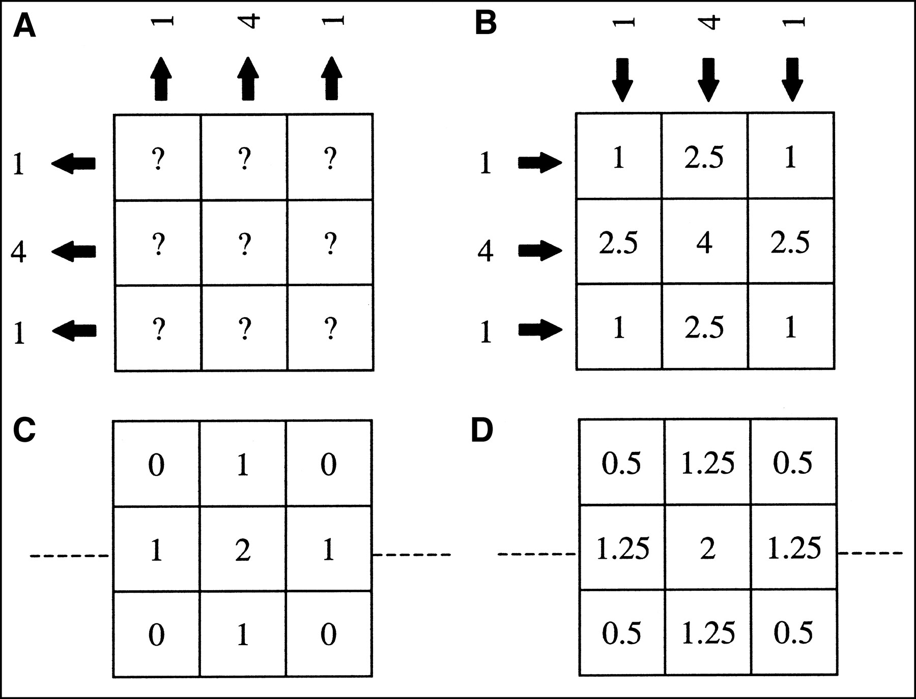
- FIGURE 8.
Blur introduced by backprojection. (A) Projection data are given. (B) Backprojection allows one to find values for 9 pixels. (C) Original image, whose projections are given in A, is shown. To compare original image and reconstructed image, image in B has been arbitrarily normalized to same maximum as original image: (D) Result is presented. Note how absolute difference between any 2 pixels is lower in D than in C.
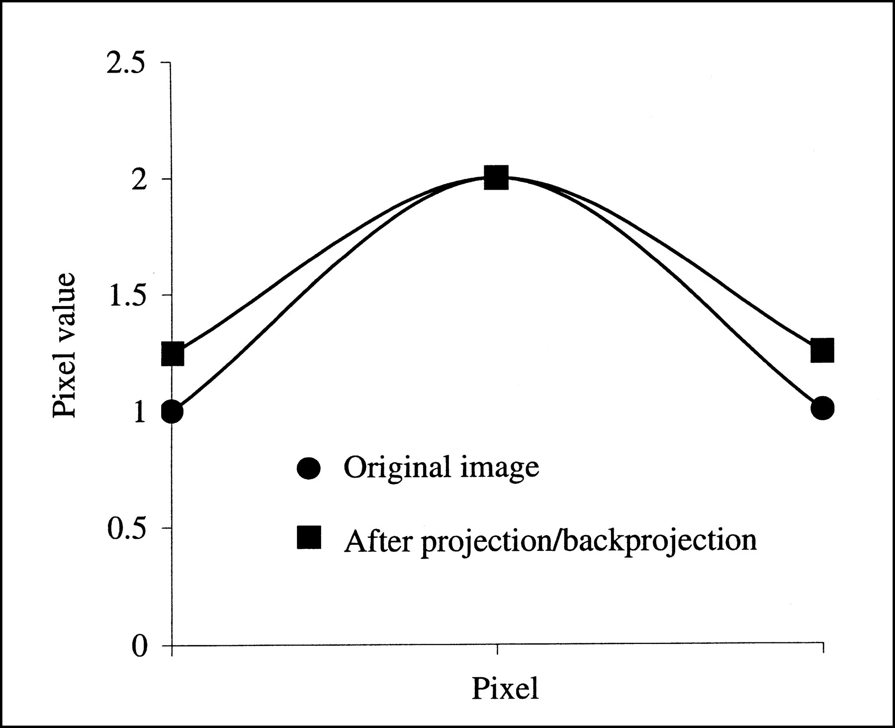
- FIGURE 9.
Activity profiles drawn along dashed lines in Figure 8. More gentle curve of profile after backprojection is illustration of blur.
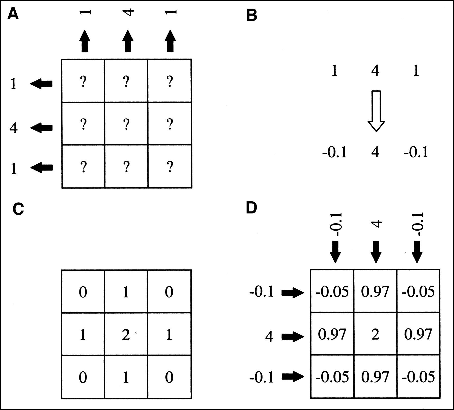
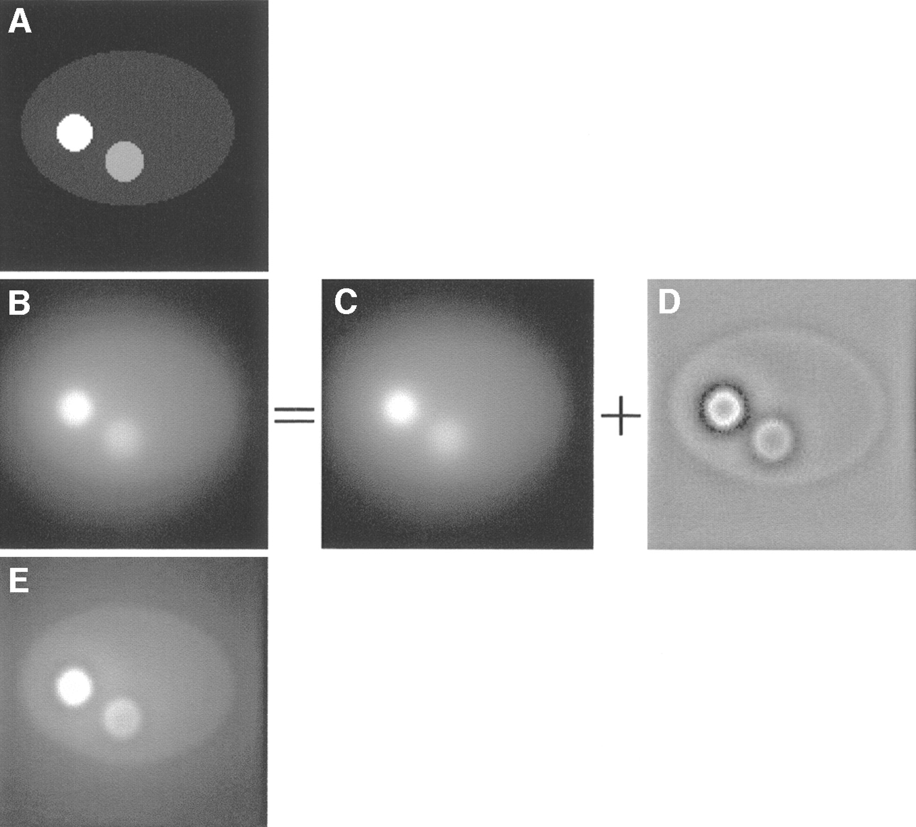
- FIGURE 10.
Simplified illustration of filtering process. (A) Model (128 × 128 pixels). (B) Image obtained after backprojection of 128 projections. (C) Low-frequency component of image presented in B. Only overall aspect of image is visible. (D) High-frequency component of image presented in B. Edges are emphasized. Dark rings correspond to negative pixel values. Sum of images in C and D yields image in B. (E) Images in C and D are added, but after C is given low weight to reduce amplitude of low-frequency component.
- FIGURE 11.
(A) Two projections are same as in Figure 8. (B) Filtering of projections using ramp filter yields negative values. (C) Original image. (D) Image obtained after backprojection of filtered projections. Note how negative and positive values substantially cancel each other, yielding result closer to original image that can be seen in Figure 8D.
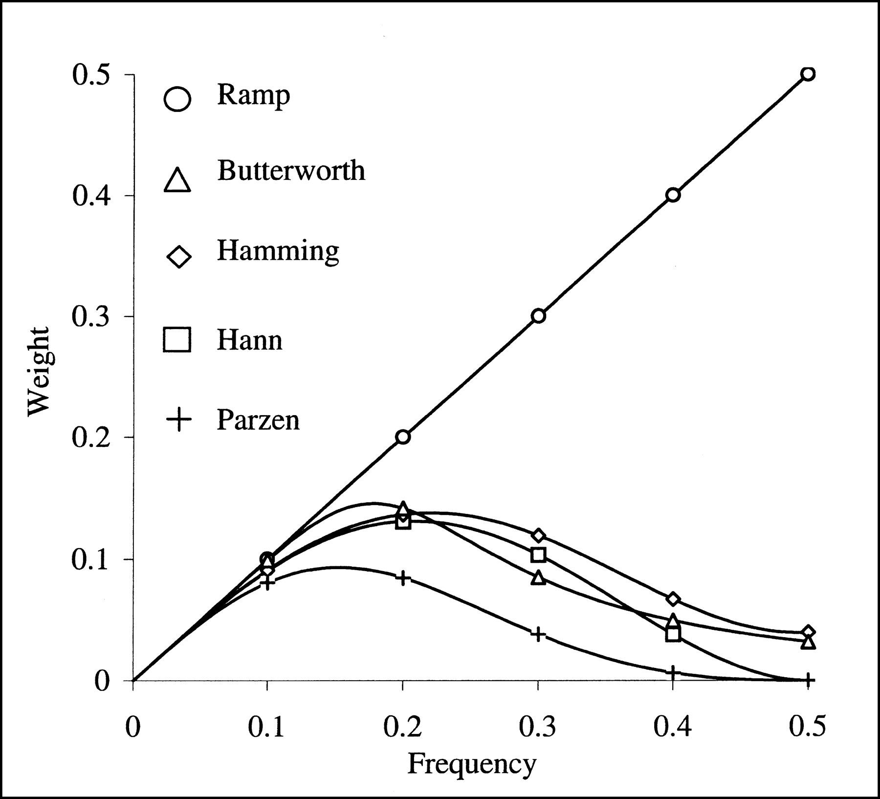
- FIGURE 12.
Some filters currently used in FBP and their shape. Value on y-axis indicates to what extent contribution of each frequency to image is modified by filters. These filters, except ramp filter, simultaneously reduce high-frequency components (containing much noise) and low-frequency component (containing blur introduced by summation algorithm).
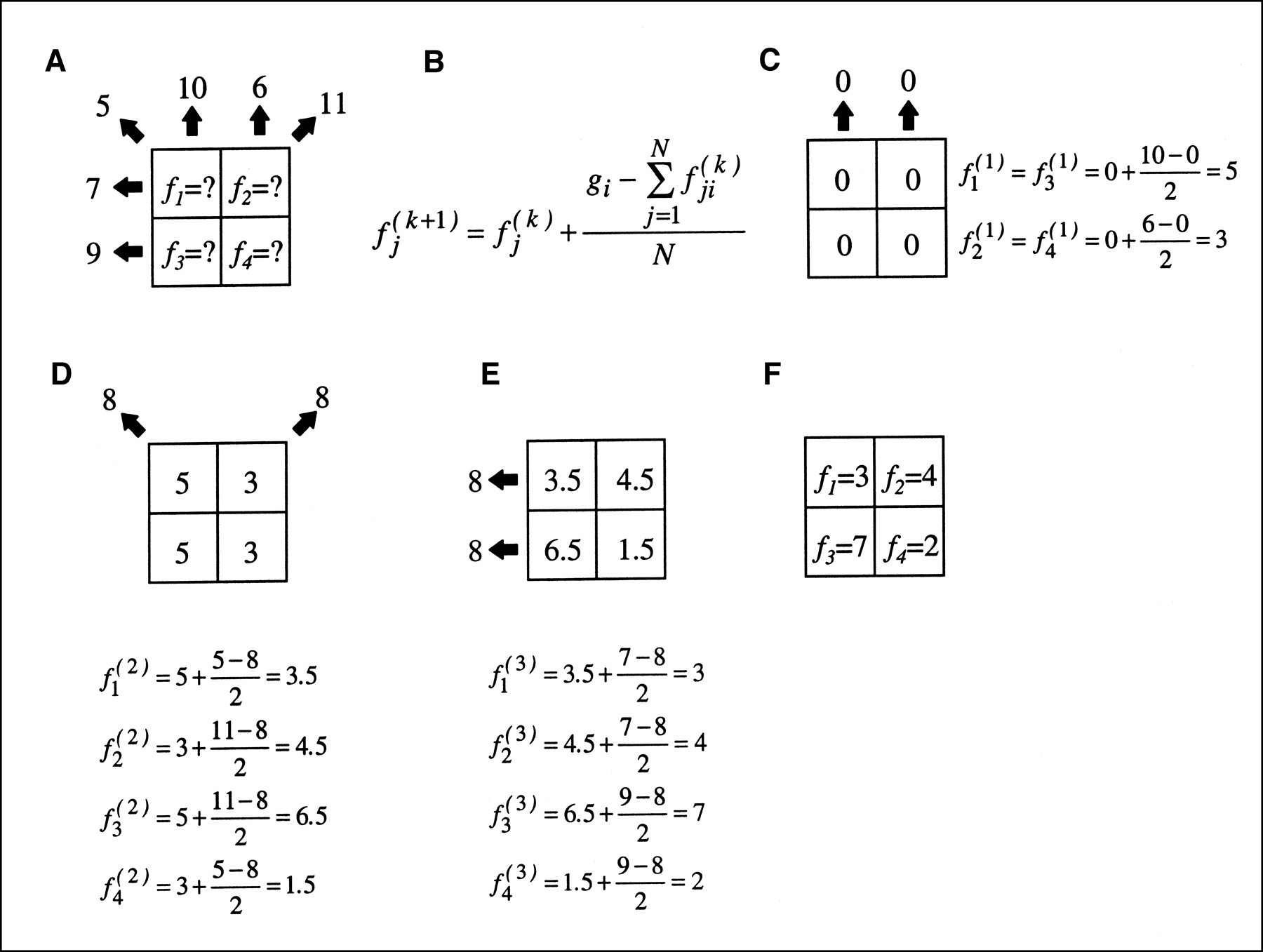
- FIGURE 13.
How ART algorithm works. (A) Problem is to find values of 4 pixels given values in 6 bins. (B) ART algorithm: Difference between estimated and measured projections is computed and divided by number of pixels in given direction. Result is added to current estimate. (C) First step: Project initial estimate (zeros) in vertical direction, apply ART algorithm, and update pixel values. Repeat this process for oblique (D) and horizontal (E) rays. (F) Solution is obtained after 1 full iteration. However, with larger images, more iterations are typically required.
- FIGURE 14.
Gradient algorithm. This plot displays difference between estimated and measured projections (vertical axis) as function of values in 2 pixels of an image. Black lines are contour lines. Goal of algorithm is to find lowest point. From initial estimate for image (point A), step along steepest descent (dashed arrow) to reach point B. Then, at B, step along steepest descent (solid arrow) to reach minimum (point C). Values for 2 pixels at location C give solution. Note that, depending on location for starting point A, minimum can be different.
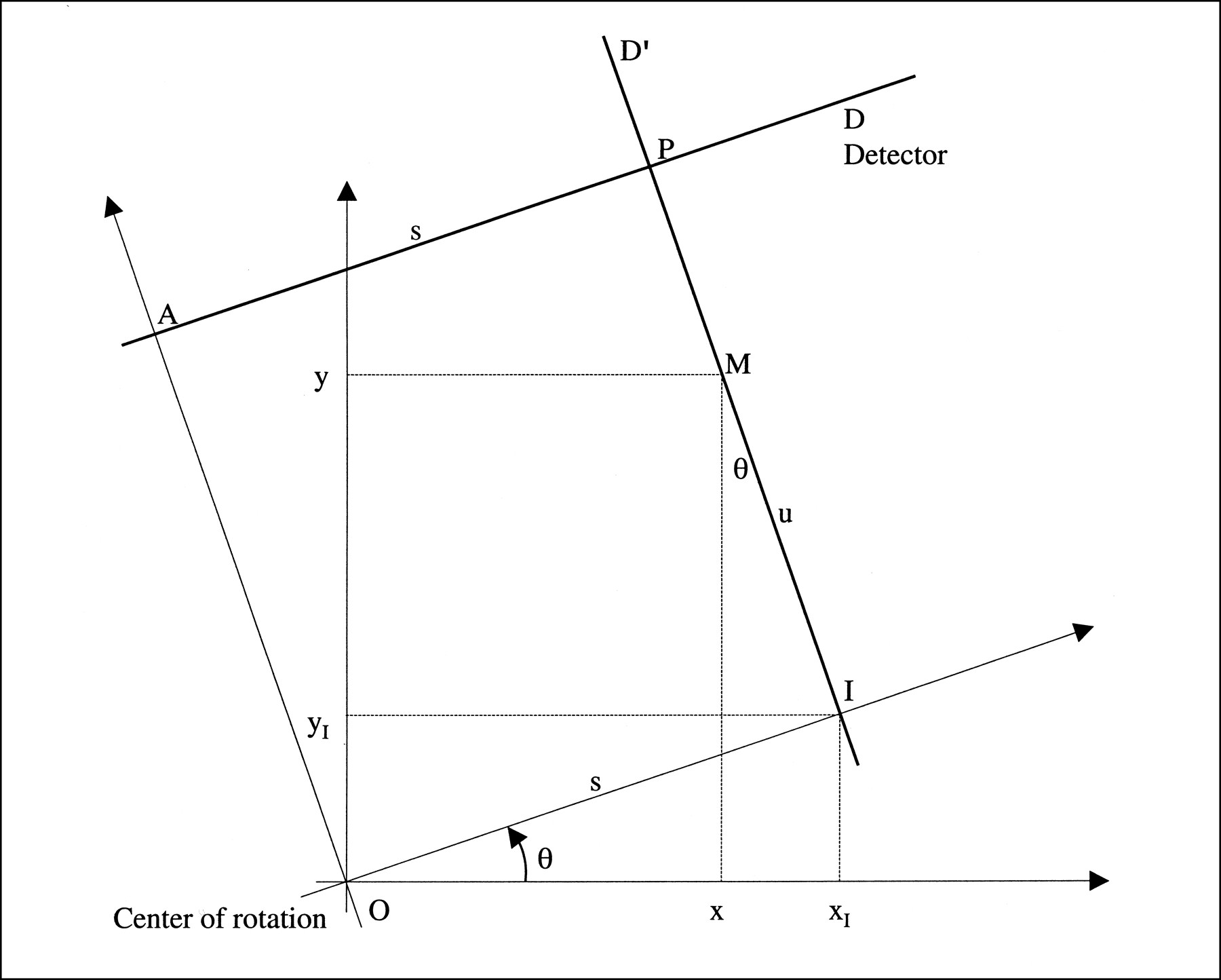
- FIGURE 15.
Geometric considerations. Point O is center of rotation of detector, and A is middle of detector line symbolized by line D. Angle θ marks angular position of detector. Line D′ is set of points M in field of view that projects perpendicularly on D in P. Distance from I to M is u. Distance from A to P is s. Note that (s, θ) are not polar coordinates of M or P.


Tables
g Vector of projection data f Vector of image data A Matrix such that g = Af aij Value of element located at ith row and jth column of matrix A i Projection subscript j Pixel subscript gi Number of counts in ith bin of a projection dataset ḡi Mean value of gi, assuming gi is a Poisson random variable fj Number of disintegrations in jth pixel of a slice f̄j Mean value of fj assuming fj is a Poisson random variable m Number of pixels n Number of bins
In this issue


Jump to section
Related Articles
Cited By...
- Scale-dependent brain age with higher-order statistics from structural magnetic resonance imaging
- Maximum-Likelihood Expectation-Maximization Algorithm Versus Windowed Filtered Backprojection Algorithm: A Case Study
- Sources of Apical Defects on a High-Sensitivity Cardiac Camera: Experiences from a Practice Performance Assessment
- Small-Animal SPECT and SPECT/CT: Important Tools for Preclinical Investigation
- SPECT/CT Physical Principles and Attenuation Correction
- Recent Advances in SPECT Imaging
- Image Reconstruction Using Filtered Backprojection and Iterative Method: Effect on Motion Artifacts in Myocardial Perfusion SPECT