


Abstract
Both the standardized uptake value ratio (SUVR) and the Logan plot result in biased distribution volume ratios (DVRs) in ligand–receptor dynamic PET studies. The objective of this study was to use a recently developed relative equilibrium–based graphical (RE) plot method to improve and simplify the 2 commonly used methods for quantification of 11C-Pittsburgh compound B (11C-PiB) PET. Methods: The overestimation of DVR in SUVR was analyzed theoretically using the Logan and the RE plots. A bias-corrected SUVR (bcSUVR) was derived from the RE plot. Seventy-eight 11C-PiB dynamic PET scans (66 from controls and 12 from participants with mild cognitive impaired [MCI] from the Baltimore Longitudinal Study of Aging) were acquired over 90 min. Regions of interest (ROIs) were defined on coregistered MR images. Both the ROI and the pixelwise time–activity curves were used to evaluate the estimates of DVR. DVRs obtained using the Logan plot applied to ROI time–activity curves were used as a reference for comparison of DVR estimates. Results: Results from the theoretic analysis were confirmed by human studies. ROI estimates from the RE plot and the bcSUVR were nearly identical to those from the Logan plot with ROI time–activity curves. In contrast, ROI estimates from DVR images in frontal, temporal, parietal, and cingulate regions and the striatum were underestimated by the Logan plot (controls, 4%–12%; MCI, 9%–16%) and overestimated by the SUVR (controls, 8%–16%; MCI, 16%–24%). This bias was higher in the MCI group than in controls (P < 0.01) but was not present when data were analyzed using either the RE plot or the bcSUVR. Conclusion: The RE plot improves pixelwise quantification of 11C-PiB dynamic PET, compared with the conventional Logan plot. The bcSUVR results in lower bias and higher consistency of DVR estimates than of SUVR. The RE plot and the bcSUVR are practical quantitative approaches that improve the analysis of 11C-PiB studies.
Pittsburgh compound B labeled with 11C (11C-PiB) is one of the most widely used compounds for in vivo detection of fibrillar β-amyloid deposition in brain (1). The spatial distribution of amyloid deposition in Alzheimer disease, mild cognitive impairment (MCI), and adults who are cognitively normal has been well characterized (2–5). The distribution volume ratio (DVR) or binding potential (DVR − 1) is usually used as an index of 11C-PiB–specific binding to tissue for quantitative measurement of β-amyloid deposition (6). In ligand–receptor dynamic PET studies, DVR can be estimated by fitting a kinetic model to the tissue kinetics with a metabolite-corrected plasma input function (7,8), where the tracer kinetic model can be a classic compartment model or a model-independent graphical analysis method and the plasma input function is the tracer radioactivity in plasma, usually measured by serial arterial blood sampling. However, quantitative PET without arterial blood sampling is more practical, and various reference tissue models have been evaluated for noninvasive quantification of 11C-PiB dynamic PET (9–14). Importantly, in these studies, the target–to–reference (cerebellum) tissue tracer concentration ratio was shown to achieve a constant at approximately 50 min after tracer injection (12,13), lending itself to pixelwise analysis using simplified, noncompartmental approaches (14). Many 11C-PiB studies have used standardized uptake value ratio (SUVR) with a reference tissue because of this method's simplicity and short scan time, in which the SUVR is calculated as target–to–reference tissue tracer concentration ratio over time frame (T0 T1) after tracer injection, where T0 and T1 are the start and end times of PET scanning.
Although there are variations in the selection of time frames (T0 T1) for SUVR measurements (15), the main disadvantage of the SUVR is the positive bias resulting in overestimation of DVR (16,17). In contrast, a commonly used Logan plot demonstrates inherent negative bias, which is attributed to noise and the target tissue tracer concentration (18–22). The linearized methods, particularly the multilinear reference tissue model (23), provide estimates of DVR similar to those from a simplified reference tissue model (SRTM) (9) yet with much higher computational efficacy. At the pixel level, PET measurements have high noise, and thus underestimation of DVR occurs with both graphical (19) and linearized methods (10,18,24). Although all of these approaches are associated with bias, and bias may be one of the limiting factors for application of the simplified quantitative methods to this tracer, bias consistency across clinical groups has not been extensively explored in 11C-PiB studies.
A novel, noninvasive, and computationally efficient graphical approach, the relative equilibrium–based graphical (RE) plot, has been recently developed for analysis of tracer kinetics, with equilibrium relative to input function (25). For reference tissue input function, target tissue tracer kinetics attain a relative equilibrium if there is a t* such that the ratio of the target to reference tissue tracer concentration is constant for t ≥ t*. In this study, the RE plot with reference tissue input was used to analyze the overestimation of DVR in SUVR measurements, develop a practical method that allows correction of the overestimation bias in SUVR, and generate DVR images that avoid the noise-induced underestimation in estimates from the Logan plot.
MATERIALS AND METHODS
Correction of DVR Overestimation in SUVR Using RE Plot with Reference Tissue Input
The inconsistent overestimation of DVR in SUVR was first demonstrated using the Logan plot with plasma input (supplemental data, available online only at http://jnm.snmjournals.org). In this section, the RE plot with reference tissue input is used to analyze the overestimation of DVR in SUVR. Let C(t) and CREF(t) be the tracer concentrations at time t in target and reference tissues, respectively. In this study, we assume that there is a time t* such that the tissue kinetics attain equilibrium relative to the reference tissue input—that is, C(t)/CREF(t) is a constant for t ≥ t*—and reference tissue input CREF(t) can be approximated by 1 exponential as CREF(t) = αeβt for t ≥ t*. For tracer kinetics that attain relative equilibrium, the RE plot with reference tissue input (25) described by Equation 1 has been proposed to simplify and improve the generation of DVR images using the conventional Logan plot with reference tissue input:
By taking derivative of both sides of Equation 1 in bilinear form and then dividing by CREF(t), we have
For the tracer delivered by bolus injection, β is negative. The θ in the RE plot is also negative, and its absolute value is positively correlated with the DVR (25). Therefore, the bias term θβ in Equation 3 is positive, and the overestimation of DVR in SUVR increases as DVR increases.
Equation 3 shows a linear relationship between θ and SUVR at a given β. We can rewrite the linear relationship between θ and SUVR as
In Equation 5, β was estimated by fitting 1 exponential to the reference tissue input CREF(t) for t ≥ t* using linear regression of time t (independent regression variable) versus the natural logarithm of CREF(t) (dependent regression variable) for each dynamic PET scan.
For the region-of-interest (ROI)–based bias correction of SUVR, the ROI-specific λ and μ were estimated by linear regression using Equation 4 with θ and SUVR from all subjects by assuming that Equation 4 holds for the whole population for a given ROI. The ROI bcSUVR for each subject was then calculated using Equation 5 with the ROI-specific λ and μ from the population and β from the subject's CREF(t).
For pixelwise bias correction of SUVR, Equation 6 was used to generate bcSUVR images for each subject:
Statistics of Linear Regression: θ = λSUVR + μ (Eq. 4)
Human 11C-PiB Dynamic PET
Study Participants
Seventy-eight 11C-PiB dynamic PET studies of nondemented older participants in the neuroimaging substudy of the Baltimore Longitudinal Study on Aging (26) were acquired. In conjunction with each 11C-PiB study, all participants received a detailed physical examination, including medical history updates and laboratory screening, neuropsychologic testing, and assessment by the Clinical Dementia Rating (CDR) (27) scale. The CDR scores were typically based on informant (spouse, child, or close friend) interviews conducted by a certified examiner. Cognitive status was determined by consensus diagnosis according to established procedures (28,29). A diagnosis of MCI was made in participants who had cognitive impairment (typically memory) but did not have functional loss in activities of daily living. Sixty-six scans from individuals with a CDR of 0 (age range at baseline scan, 55.7–92.1 y; mean age ± SD, 77.6 ± 6.9 y) were classified as the control group, and 12 scans from individuals with a CDR of 0.5 (age range at baseline scan, 77.2–89.5 y; mean age ± SD, 83.5 ± 4.3 y) were classified as the MCI group. In this study, we considered a CDR of 0.5 as indicative of MCI, but only 3 individuals actually met the consensus criteria for MCI.
11C-PiB Dynamic PET
All dynamic PET studies were obtained on an Advance scanner (GE Healthcare). PET was started immediately after an intravenous bolus tracer injection (543.5 ± 29.7 MBq; range, 442.9–605.3 MBq) with a high specific activity (236.6 ± 145.4 GBq/μmol; range, 36.1–1,005.4 GBq/μmol) at the time of injection of 11C-PiB. There were no significant differences in 11C-PiB dose or specific activity among cognitively impaired and cognitively normal older adults (P > 0.05). Dynamic PET data were collected in 3-dimensional acquisition mode according to the following protocol: 4 × 0.25, 8 × 0.5, 9 × 1, 2 × 3, and 14 × 5 min (90 min total, 37 frames). To minimize head motion during PET, all participants were fitted with thermoplastic face masks. The reconstruction of dynamic PET images was described in our previous studies (10).
Structural MRI and ROI Definition
Structural MR images for anatomic localization were obtained on a Signa 1.5-T (GE Healthcare) or Intera 3.0-T (Phillips) scanner using a spoiled gradient-recalled acquisition sequence (124 slices with a 256 × 256 image matrix, pixel size of 0.94 × 0.94 mm, and slice thickness of 1.5 mm). MR images were typically obtained on the same visit, but a major renovation of the MRI research scanners coincided with 11C-PiB imaging studies. Although 61 MR images were acquired at the time of the PET scan, 15 were obtained within 1.8 y (SD, 0.8 y; range, 1–4.1 y) of the PET scan. Two additional MR images were acquired 10.5 and 11.8 y before the PET scans because of medical issues that prevented concurrent MRI assessments. MR images were coregistered to the mean image of the first 20 min of dynamic PET scanning using SPM2 (Statistical Parametric Mapping software; Wellcome Department of Cognitive Neurology) with the mutual-information method. In addition to the reference region (cerebellar cortex), 14 ROIs were manually drawn on the coregistered MR images (10,12,13) and copied to the dynamic PET images to obtain ROI time–activity curves for kinetic analysis. The ROIs were also applied directly to parametric images for estimation of DVRs.
Evaluation of RE Plot and Parameter Estimation
The evaluation of assumptions for the RE plot is provided in the supplemental data. The single t* value used in the RE and Logan plots and SUVR (supplemental data) for all subjects were determined at 52.5 min after tracer injection, corresponding to the last 8 time frames, from 50 to 90 min of dynamic scanning. DVRs from the RE plot, the Logan plot with reference tissue input (10,11,25) (hereafter, the Logan plot) (supplemental data), and the SUVR were calculated from ROI kinetics. Subsequently, parametric images from pixelwise kinetics were obtained using the RE and Logan plots, the SUVR and bcSUVR, and the SRTM. The ROIs from the parametric images were then compared with the DVRs from ROI kinetics. The estimates of DVR from the low noise levels of ROI time–activity curves were used as a reference in this study. Mean parametric images for the control and the MCI groups were then generated using SPM2. The spatial normalization parameters determined by the mean image of the first 20 min of dynamic PET scanning were applied to all parametric images (10).
All parameter estimation methods for ROI kinetic analysis and parametric image generation were written in MATLAB (The MathWorks Inc.) and implemented on a PWS690 workstation (Dell).
Evaluation of Assumptions for Bias-Corrected SUVR
The values of β obtained by fitting 1 exponential to the reference tissue input CREF(t) for t ≥ t* = 52.5 min were compared between patient and control groups using the statistical t test.
To evaluate the assumption that CREF(t) can be approximated by 1 exponential as CREF(t) = αeβt for t ≥ t* = 52.5 min, CREF(t) was fitted not only by 1 exponential but also by multiexponentials as CREF(t) = α0 +
The assumption of the linear relationship between θ and SUVR was evaluated by applying linear regression of θ (y-variable) versus SUVR (x-variable) for each ROI time–activity curve over all subjects, where θ was estimated by the RE plot with t* = 52.5 min.
RESULTS
Validation of Assumptions for Bias-Corrected SUVR
We verified the 2 assumptions used to derive the bcSUVR from the RE plot. The first assumption is that 1-exponential clearance occurs after t* for reference tissue (cerebellum) kinetics. The cerebellum time–activity curves were well fitted by an exponential function at t ≥ t* = 52.5 min. The R2 of the linear regression of time t versus the natural logarithm of cerebellum time–activity curves was 0.790 ± 0.196 and 0.867 ± 0.071 for controls and the MCI group, respectively. The β-values, the 1-exponential clearance rates of tracer concentration in cerebellum, were 0.007 ± 0.003 min−1 in controls and 0.008 ± 0.002 in the MCI group. They were not significantly different between these 2 groups (P = 0.33). The value of the Akaike information criterion calculated from 1-exponential fitting (−87.47 ± 6.34) was significantly lower than that obtained from multiexponential fitting (−85.88 ± 6.98; paired t test, P = 0.009), and the results demonstrate that the 1-exponential model better predicts or fits reference tissue input CREF(t) for t ≥ t* = 52.5 min.
The second assumption is that there is a linear relationship between SUVR and θ. As shown for a representative ROI, the posterior cingulate cortex, there was a highly linear relationship between SUVR and bias correction factor θ, where absolute value of the correction factor θ increases as SUVR increases (supplemental data; Fig. 3). The values for λ and μ, that is, the slope and the intercept of the linear regression of θ versus SUVR, for all 14 ROIs are listed together with R2 values in Table 1. The percentage coefficient of variation (=100[SD/mean]) of λ was 5.6%. Because of this low variation of λs in different ROIs, there was no significant difference between mean λ and ROI-specific λ for any ROIs (P = 0.33 ± 0.23; range, 0.06–0.75) except the putamen (P = 0.04).
Bias and Bias Correction of SUVR in ROI Kinetics
Inconsistent overestimation of the DVR in SUVR between controls and MCI subjects is illustrated in Figure 1A. The SUVR overestimation in this figure is calculated as percentage bias (Bias%) relative to the DVR estimated from ROI time–activity curves using the Logan plot. The overestimation of DVRs in SUVR ranges from 16% to 32% in the MCI group and is significantly higher (on average 1.73 times higher) than in controls in all but 4 ROIs (mesial temporal, occipital, pons, and white matter).
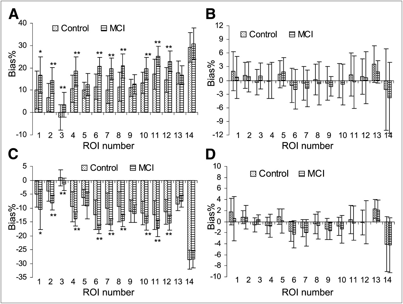
Variability of Bias% in ROI DVR estimates relative to DVRs from Logan plot with reference tissue input and ROI time–activity curves between MCI and control groups: SUVR (A), bcSUVR (B), DVR from parametric images generated by Logan plot (C), and DVR from RE plot (D). Bias% = 100(DVR/DVR(Logan plot with ROI time–activity curves) − 1). Regions of interest (ROIs) are numbered as 1, caudate; 2, putamen; 3, thalamus; 4, lateral temporal; 5, mesial temporal; 6, orbital frontal; 7, prefrontal; 8, superior frontal; 9, occipital; 10, parietal; 11, anterior cingulate; 12, posterior cingulate; 13, pons; and 14, white matter. For RE plot, DVRs from ROI time–activity curves are identical to those from DVR images. Although group differences in Bias% are detected for SUVR and DVR images generated by Logan plot from high-noise-pixel time–activity curves, bcSUVR and DVRs from the RE plot do not show any group differences. *0.02 ≤ P ≤ 0.05. **P < 0.01.
The bcSUVR was developed to address the inconsistency bias of the SUVR. Figure 1B shows that this method is associated with minimal bias (Bias% ≤ 2.0% for all ROIs, except 3.6% for pons) relative to the DVRs estimated from ROI time–activity curves using the Logan plot and that there is no difference between the MCI group and control group in Bias% (statistical P value, 0.46 ± 0.28; range, 0.08 to 0.94). Figures 2A and 2B show that, after using the bcSUVR, the linear relationship between the SUVR and DVR from ROI time–activity curves using the Logan plot improved, because the slope of the regression line changed from 1.37 to 1.02 and R2 increased from 0.94 to 0.96.
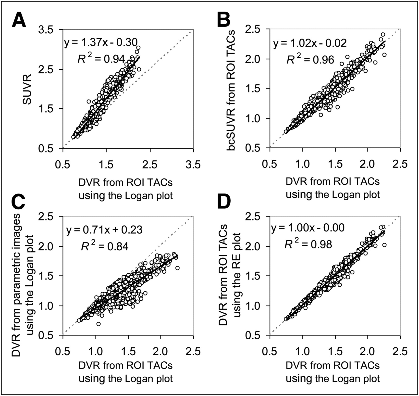
Linear correlations between DVR estimates from ROI time–activity curves using Logan plot and SUVR (A), bcSUVR (B), DVR from parametric images generated by Logan plot (C), and DVRs from parametric images generated by RE plot (D). TAC = time–activity curve.
SUVR, bcSUVR, and DVR Images
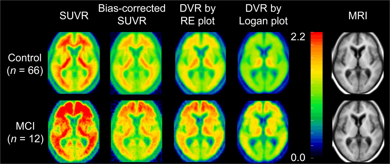
The constants for generating the bcSUVR images, λ and μ, are −39.97 and 34.71, respectively (Table 1). The mean images of SUVR, bcSUVR, and DVRs generated by the RE and Logan plots are shown in Figure 3. As expected, there is overestimation in the SUVR images and noise-induced underestimation in the DVR images generated by the Logan plot. Because the ROIs from SUVR images are identical to those from ROI time–activity curves, the overestimation of DVR in SUVR images was the same as shown in Figures 1A and 2A. The bcSUVR images are comparable to the images generated by the RE plot. There was a highly linear correlation between the ROI values from bcSUVR images and the bcSUVR calculated from ROI time–activity curves: (bcSUVR image) = 0.96DVR(bcSUVR ROI time–activity curves) + 0.05, with R2 = 0.98. As compared with the DVRs from the RE plot or the Logan plot with ROI time–activity curves, the Bias% of bcSUVR was less than ±6% for ROIs including the cortex, striatum, and pons; approximately −11% in the thalamus; and approximately 8% in white matter. In addition, no significant difference in Bias% of bcSUVR was observed between the MCI group and controls. For the Logan plot, the DVR ROI values obtained directly from the parametric DVR images were lower by approximately 12.2% (excluding white matter) than those from the ROI time–activity curves from low noise levels. The underestimation in the DVR images in the MCI group was significantly higher than that of controls in all but 4 ROIs (mesial temporal, occipital, pons, and white matter) (Fig. 1C). For the RE plot, the DVR estimates from ROI time–activity curves were identical to those obtained by applying ROIs to DVR images. Therefore, the noise-induced underestimation in the DVR images generated by the Logan plot in both control and MCI groups was removed completely using the RE plot (Figs. 1D, 2C, and 2D).

Mean of parametric images generated using SUVR, bcSUVR, and DVR images generated by RE plot and Logan plot in MCI and control groups. Mean MR image is provided for anatomic information.
Comparison of DVR Estimates Between Control and MCI Groups
The comparison of ROI estimates of DVR between control and MCI groups is summarized in Supplemental Table 2. The DVR estimates from all methods were consistently higher in the MCI group than in controls (P < 0.05) for all ROIs except for mesial temporal and occipital cortex, pons, and white matter. In comparison to the DVRs from the Logan plot with ROI time–activity curves, the contrast between DVR in MCI and control groups was increased when quantitated by SUVR and decreased when parametric images were generated by the Logan plot. On the basis of the DVRs estimated from the ROI time–activity curves using the Logan plot, the DVRs in the following ROIs were higher (P < 0.05) in the MCI group than in the control group: frontal (orbital, prefrontal, and superior), by 36.1%; cingulate (anterior, and posterior), by 31.7%; parietal, by 20.8%; lateral temporal, by 20.1%; striatum (caudate, putamen), by 26.2%; and thalamus, by 10.6%. In contrast, the difference between MCI and control groups was artificially increased by 8.5% for SUVR and decreased by 5.6% for the parametric DVR images generated by the Logan plot. As demonstrated in Supplemental Table 2, for both control and MCI groups, the DVRs estimated by bcSUVR from ROI time–activity curves, bcSUVR images, and RE plot are similar to those from the Logan plot from ROI time–activity curves. The percentage differences in DVRs between MCI and control groups in ROIs (mesial temporal, pons, and white matter) were consistent across all methods, with less than 6% absolute difference, and were of no statistical significance (P > 0.30).
DISCUSSION
In this study, we proposed that the bcSUVR and the RE plot improve the estimates of DVR from SUVR and the Logan plot, respectively. While the bcSUVR allows simplification of 11C-PiB dynamic PET data acquisition and quantification, the RE plot needs to be applied to the full dynamic PET data. SUVR is associated with positive bias observed with 11C-PiB (13,15) and with neuroreceptor ligands (17,35,36). Although this bias has been analyzed by compartmental modeling techniques (16,17), so far no approaches have been developed for mitigating such bias. The recently developed relative equilibrium-based graphical plot, the RE plot, was used to derive a correction factor that is able to mitigate the known positive bias associated with SUVR (25). Because the method for bcSUVR is based on the parameters of λ and μ estimated from a population, the generalizability of the method was validated by a cross-validation study within our dataset (supplemental data).
Quantification of the full dynamic PET dataset can also lead to inconsistent bias, as demonstrated by the DVR images generated by the Logan plot. Noise-induced underestimation is also observed in the DVR images generated by the SRTM with the conventional multilinear regression method (24). In fact, for ROI 11C-PiB kinetics of low noise levels, it was reported that the SRTM, 2-parameter SRTM, multilinear reference tissue model 2, and Logan plot provide similar DVR estimates (10,14). In this study, we also found that the DVRs from the SRTM with ROI kinetics were as close to the DVRs from the RE plot as DVR(SRTM with ROI time–activity curves) = 1.03DV(RE plot) − 0.07 (R2 = 0.96).
Both the RE plot and the bcSUVR, as well as SUVR, require the presence of equilibrium relative to reference tissue kinetics for t ≥ t*. Because it may take longer to achieve relative equilibrium for tissues with lower clearance rates or higher DVRs, the t* is likely to be determined by the ROI kinetics from older subjects and MCI patients. Here, we have validated that t* occurs at 52.5 min after tracer injection in populations including MCI subjects and controls with age ranges from 77.2 to 89.5 y and a maximum ROI DVR as high as 2.265. The onset of the relative equilibrium t* at 40–50 min was demonstrated in other 11C-PiB studies, including those with controls and MCI and AD patients (12,13,15). As such, t* = 52.5 min corresponding to dynamic PET scan frames starting from 50 min after tracer injection is an appropriate value for the RE plot and bcSUVR estimation of DVR in 11C-PiB PET studies. Relative equilibrium tracer kinetics were also observed in 11C-raclopride for dopamine D2-like receptor imaging (17,25), 2-(1-{6-[(2-18F-fluoroethyl)(methyl)amino]-2-naphthylethylidene) malononitrile} (18F-FDDNP) for imaging β-amyloid plaques and neurofibrillary tangles (37), and 18F-florbetapir and 18F-florbetaben for imaging β-amyloid (38,39). As such, the RE plot and bcSUVR methods are applicable to these tracer kinetics.
One limitation of this population-based approach is that the correction factors λ and μ obtained here may not be applicable to different populations such as AD patients or to data acquired on different scanners using different acquisition or image reconstruction protocols. However, once the bcSUVR method is carefully validated using the RE plot on the full dynamic PET scan dataset of a population of interest, it can then be used in simplified PET protocols with short acquisitions applied to individuals from that population.
CONCLUSION
We have theoretically analyzed inconsistent overestimation of DVR in SUVR and the noise-induced underestimation of DVR by the Logan plot and then demonstrated them on 11C-PiB studies of nondemented older adults. We propose that bcSUVR derived from the RE plot can simplify both clinical and research 11C-PiB data quantification. The RE plot and bcSUVR are associated with low bias, high consistency, and high computational efficiency in quantification of 11C-PiB retention. Both of these methods improve the quantification of DVR estimates compared with the Logan plot and the SUVR, 2 frequently used methods for assessment of β-amyloid burden.
DISCLOSURE STATEMENT
The costs of publication of this article were defrayed in part by the payment of page charges. Therefore, and solely to indicate this fact, this article is hereby marked “advertisement” in accordance with 18 USC section 1734.
Acknowledgments
We thank the cyclotron staff, PET staff, and MRI staff of the Johns Hopkins Medical Institutions and Andrew H. Crabb for data transfer and computer administration. This study was supported in part by the Intramural Research Program of the NIH and by the National Institute on Aging (NIA) (R&D contracts N01-AG-0012 and N01-AG-3-2124). No other potential conflict of interest relevant to this article was reported. This work was presented in part at the 56th Society of Nuclear Medicine conference, June 13–17, 2009, Toronto, Canada, and at the 57th Society of Nuclear Medicine conference, June 5–9, 2010, Salt Lake City, Utah.
Footnotes
Published online Mar. 13, 2012.
- © 2012 by the Society of Nuclear Medicine, Inc.
REFERENCES
- Received for publication August 30, 2011.
- Accepted for publication December 12, 2011.


Jump to section
Related Articles
Cited By...
- Voxelwise Relationships Between Distribution Volume Ratio and Cerebral Blood Flow: Implications for Analysis of {beta}-Amyloid Images
- Quantitative Analysis of Amyloid Deposition in Alzheimer Disease Using PET and the Radiotracer 11C-AZD2184
- Longitudinal Amyloid Imaging Using 11C-PiB: Methodologic Considerations