


Abstract
The aim of the present study was to define the optimal analytic method to derive accurate and reliable serotonin transporter (SERT) receptor parameters with 11C-3-amino-4-(2-[(dimethylamino)methyl]phenylthio)benzonitrile (11C-DASB). Methods: Nine healthy subjects (5 females, 4 males) underwent two 11C-DASB PET scans on the same day. Five analytic methods were used to estimate binding parameters in 10 brain regions: compartmental modeling with 1- and 2-tissue compartment models (1TC and 2TC), data-driven estimation of parametric images based on compartmental theory (DEPICT) analysis, graphical analysis, and the simplified reference tissue model (SRTM). Two variations in the fitting procedure of the SRTM method were evaluated: nonlinear optimization and basis function approach. The test/retest variability (VAR) and intraclass correlation coefficient (ICC or reliability) were assessed for 3 outcome measures: distribution volume (VT), binding potential (BP), and specific to nonspecific equilibrium partition coefficient (V3″). Results: All methods gave similar values across all regions. The variability of VT was excellent (≤10%) in all regions, for the 1TC, 2TC, DEPICT, and graphical approaches. The variability of BP and V3″ was good in regions of high SERT density and poorer in regions of moderate and lower densities. The ICC of all 3 outcome measures was excellent in all regions. The basis function implementation of SRTM demonstrated improved reliability compared with nonlinear optimization, particularly in moderate and low-binding regions. Conclusion: The results of this study indicate that 11C-DASB can be used to measure SERT parameters with high reliability and low variability in receptor-rich regions of the brain, with somewhat less reliability and increased variability in regions of moderate SERT density and poor reproducibility in low-density regions.
Recently, Wilson et al. (1) and Ginovart et al. (2) introduced 11C-3-amino-4-(2-[(dimethylamino)methyl]phenylthio)benzonitrile (11C-DASB), a new PET radiotracer to image the serotonin transporter (SERT). 11C-DASB has emerged as the current PET radiotracer of choice to quantify SERT in clinical studies, such as methylenedioxymethamphetamine users (3), patients with depression (4), and patients with schizophrenia (5). Despite this the test/retest reproducibility of 11C-DASB binding parameters estimates in the human brain have not been reported yet.
The aim of the present study was to evaluate the reproducibility of SERT receptor parameters' derivation with 11C-DASB in regions of high, moderate, and low SERT density. Nine healthy volunteers were studied twice on the same day after injection of 11C-DASB. Five approaches were compared for measurement of SERT receptor parameters: kinetic 1- and 2-tissue compartment (1TC and 2TC) models, a simplified reference tissue model (SRTM) (6), DEPICT (7), and graphical analysis (8). Three outcome measures were compared: total distribution volume (VT), binding potential (BP), and specific-to-nonspecific equilibrium partition coefficient (V3″). The comparison included the following attributes of the outcome measures: their identifiability, which describes the degree of certainty in parameter estimation, as well as the variability and reliability, which were assessed with test/retest reproducibility studies.
MATERIALS AND METHODS
Human Subjects
The study was approved by the Institutional Review Boards of the New York State Psychiatric Institute and Columbia Presbyterian Medical Center. Nine healthy volunteers participated in this study (age, 29 ± 8 y; range, 19–40 y, with these and subsequent values given as mean ± SD, 4 males, 5 females). All scans were performed between June 5, 2002, and March 10, 2003. All subjects recruited into the study are included in the analysis. The absence of pregnancy, medical, neurologic, and psychiatric history (including alcohol and drug abuse) was assessed by history, review of systems, physical examination, routine blood tests including pregnancy test, urine toxicology, and electrocardiogram. Subjects provided written informed consent after receiving an explanation of the study.
Radiochemistry
The standard DASB and precursor desmethyl DASB were a gift from the University of Toronto. Preparation of 11C-DASB followed the literature procedure, with some modifications (1,9).
The chemical purity of 11C-DASB was 98.9% ± 1.1% and the radiochemical purity was 94.8% ± 2.5%.
PET Protocol
Each subject underwent 2 scans with 11C-DASB on the same day. An arterial catheter was inserted into the radial artery after completion of the Allen test and infiltration of the skin with 1% lidocaine. A venous catheter was inserted in a forearm vein on the opposite side. Head movement minimization was achieved with a polyurethane head immobilization system (Soule Medical) (10). PET was performed with the ECAT EXACT HR+ (Siemens/CTI). A 10-min transmission scan was obtained before radiotracer injection. 11C-DASB was injected intravenously over 45 s. Emission data were collected in 3-dimensional mode for 120 min as 21 successive frames of increasing duration (3 × 20 s, 3 × 1 min, 3 × 2 min, 2 × 5 min, 10 × 10 min). Subjects were allowed to rest outside of the camera for 30–45 min between the 2 injections.
Input Function Measurement
After radiotracer injection, arterial samples were collected every 10 s with an automated sampling system for the first 2 min and manually thereafter at longer intervals. A total of 32 samples were obtained per scan. After centrifugation (10 min at 1,800g), plasma was collected in 200-μL aliquots and activities were counted in a γ- counter (model 1480 Wizard 3M Automatic γ-Counter; Wallac).
Six samples (collected at 16, 30, 50, 70, 90, and 120 min) were further processed by high-pressure liquid chromatography to measure the fraction of plasma activity representing unmetabolized parent compound (9).
A biexponential function was fitted to the 6 measured unmetabolized fractions and used to generate a continuous measure of the parent fraction in plasma. The smallest exponential of the unmetabolized fraction curve, λpar, was constrained to the difference between λcer, the terminal rate of washout of cerebellar activity, and λtot, the smallest elimination rate constant of the total plasma activity (11).
The input function, the initial distribution volume (Vbol, L), and the clearance of the parent compound (CL, L/h) were calculated following published methodology (9,12).
The plasma free fraction (f1) was determined as previously described (5,13).
MRI Acquisition and Segmentation Procedures
MR images were acquired and segmentation was performed following previously published methods (5,14).
Image Analysis
Images were reconstructed to a 128 × 128 × 63 matrix (voxel size of 1.7 × 1.7 × 2.4 mm) with attenuation correction using the transmission data and a Shepp 0.5 filter. Reconstructed image files were then processed with the image analysis software MEDx (Sensor Systems, Inc.). All frames were realigned to a frame of reference, using a least-squares algorithm for within-modality coregistration (automated image registration [AIR]) (15). After frame-to-frame registration, the 21 frames were summed to generate a single data volume, which was coregistered to the MRI dataset using AIR (15). The spatial transformation derived from the summed PET registration procedure was then applied to each registered frame. Thus, each PET frame was resampled in the coronal plane to a voxel volume of 1.5 × 0.9 × 0.9 mm3.
Regions of interest (ROIs, n = 10) and region of reference (cerebellum) boundaries were drawn on the MR image according to criteria derived from brain atlases (16,17) and published reports (18–21). A segmentation-based method was used for the neocortical regions and a direct identification method was used for the subcortical regions (14).
The neocortical regions (n = 6) were as follows: dorsolateral prefrontal cortex (DLPFC, 30,753 ± 7,102 mm3), medial prefrontal cortex (MPFC, 7,268 ± 3,275 mm3), orbitofrontal cortex (OFC, 16,099 ± 3,535 mm3), anterior cingulate cortex (ACC, 4,752 ± 2,223 mm3), temporal cortex (TC, 54,225 ± 10,743 mm3), and occipital cortex (OC, 43,804 ± 8,066 mm3).
The subcortical regions (n = 5) included striatum (STR, 21,607 ± 3,340 mm3), thalamus (THA, 9,925 ± 1,636 mm3), midbrain (MID, 6,796 ± 623 mm3), medial temporal lobe (MTL, 24,919 ± 2,923 mm3; a spatially weighted average of 5 limbic structures, the uncus, amygdala, entorhinal cortex, parahippocampal gyrus, and hippocampus), and cerebellum (CER, 35,281 ± 12,200 mm3). For bilateral regions, right and left values were averaged. The ROIs were a priori divided into 3 categories: regions with high SERT densities (MID, THA, STR), regions of moderate density (MTL and cingulate), and regions of low density (neocortical regions).
The contribution of total plasma activity to the regional time–activity data was calculated assuming a 5% blood volume in the ROIs (22), and tissue activities were calculated as the total regional activities minus the plasma contribution.
Derivation of Distribution Volumes
Kinetic Analysis.
For the kinetic analysis, both a 2-compartment model (i.e., 1TC) and a 3-compartment model (i.e., 2TC) were used. The 2TC model included the arterial plasma compartment (Ca), the intracerebral free and nonspecifically bound compartment (nondisplaceable compartment (C2), and the specifically bound compartment (C3). The 1TC model included the arterial plasma compartment (Ca) and 1 tissue compartment (CT), which includes C2 and C3. The total regional distribution volume (VT, mL g−1) was defined as the ratio of the tracer concentration in the region to the metabolite corrected plasma concentration at equilibrium: Data were fitted to the solutions of differential equations (23), and VT was derived via a nonlinear regression using a Levenberg–Marquart least-squares minimization procedure (24), implemented in MATLAB (The Math Works, Inc.), and was used for the1TC model. For the 2TC, sequential quadratic programming with bound (nonnegativity) constraint, also implemented in MATLAB, was applied. The constraint was used because we found, as previously reported by others (2), that an unconstrained 2TC failed to reliably converge. For each of these, the squared residuals in the least-squares procedure were weighted in proportion to frame duration.
DEPICT Analysis.
DEPICT (7) is a data driven method of parameter estimation that employs the basis pursuit concept (25). This method uses a basis function fitting procedure (26,27), in which an arbitrary number of basis functions can be used to fit the data due to an additional penalty term in the cost function that induces a sparse representation. DEPICT can be applied to plasma input or reference region input models, but only the plasma input models are presented here. The DEPICT VT is derived simply from the integral of the estimated impulse response function. DEPICT was implemented with 30 kinetic basis functions whose exponential coefficients ranged from 0.6 to 0.014 min−1. The relaxation parameter was fixed at a single value for all analyses based on an assessment of the leave-one-out cross-validation cost functions for all datasets. Again, data were weighted in proportion to frame duration.
Graphical Method.
Graphical determination of VT was performed by the method of Logan et al. (8). The determination of t*, the time from which the regression was computed, was performed by visual inspection.
Model Order and Goodness of Fit.
For the 1TC and 2TC, goodness of fit of models with different levels of complexity were compared using the Akaike Information Criterion (AIC) (28) and the F test (29,30). DEPICT automatically determines model order as part of the fitting procedure based on the number of components that make a substantial contribution to the impulse response function.
Derivation of SERT Parameters
Derivation of SERT parameters was based on the following assumptions: (i) because of the negligible density of SERT in the cerebellum (31–33), cerebellum VT was assumed to be representative of equilibrium nonspecific binding; (ii) the nonspecific binding did not vary significantly between regions.
The binding potential (BP) (22) was derived as the difference between VT in the ROI (VT ROI) and VT in the cerebellum (VT CER), the reference region. The relationship between BP and SERT receptor parameters is given by (34): where Bmax is the regional concentration of SERT (nmol/L), and Kd is the in vivo affinity of the tracer for SERT (nmol/L).
For all plasma input methods, the specific-to-nonspecific equilibrium partition coefficient (V3″) was derived as the ratio of BP to VT CER. The relationship between V3″ and SERT receptor parameters is given by (34): where f2 is the free fraction of the nonspecific distribution volume in the brain (f2 = f1/VT CER).
V3″ was also estimated by the simplified reference tissue method (SRTM) (6). SRTM uses assumptions (i) and (ii) to infer a functional relationship between a reference region (cerebellum) and an ROI. Because this method uses only brain data and not plasma data, V3″ is the only receptor-related parameter that can be estimated.
SRTM was applied without blood volume correction, the setting in which it would most typically be used. Two implementations of SRTM were tested. The first used an iterative optimization algorithm based on the Levenberg–Marquart procedure with fitting weights proportional to frame duration. The second implementation used a basis function approach implemented as described with 100 kinetic basis functions whose exponential coefficients ranged from 0.6 to 0.014 min−1 (26).
Evaluation of Methods
Results were evaluated according to 2 criteria: variability and reliability.
Variability.
The test/retest variability (VAR) was calculated as the absolute value of the difference between the test and retest, divided by the mean of the test and retest values.
Reliability.
To evaluate the within-subject variability relative to the between-subject variability, both within-subject SD (WSSD) and between-subject SD (BSSD) were calculated and expressed as percentage of mean value (WS %CV and BS %CV, where CV is coefficient of variation). The reliability of the measurements was assessed by the intraclass correlation coefficient (ICC) calculated as (35): where BSMSS is the mean sum of square between subjects and WSMSS is the mean sum of square within subjects. This statistic estimates the relative contributions of between- and within-subject variability and assumes values from −1 (i.e., BSMSS = 0) to 1 (identity between test and retest, i.e., WSMSS = 0).
In addition, the numeric identifiability of the total distribution volume was examined for the 1TC and 2TC models. VT identifiability statistics were derived as the square root of the quadratic form ∇k(VT)′C ∇k(VT), where ∇k(VT) is the gradient of the outcome measure VT with respect to the rate constants and C is the covariance matrix (inverse of the Fisher information matrix) of the rate constants (29,30), expressed as % of the respective parameters (%CV).
Statistical Analysis
The average of the test and retest values was calculated for each subject (n = 9) and the results are given as mean ± SD of these 9 average measurements. This allows for estimation of the variability in the population (i.e., between-subject SD). When the SD refers to variability between experiments rather than between subjects, the SD is followed by n = 18. Dependent variables were analyzed using repeated-measures ANOVA (RM ANOVA). A 2-tailed probability value of 0.05 was selected as the significance level.
RESULTS
Injected Dose
The injected dose (529.1 ± 62.9 MBq, n = 18), injected mass (5.4 ± 2.2 μg, n = 18), and specific activity (35.37 ± 21.94 GBq/μmol, n = 18) did not differ between the test and retest conditions (RM ANOVA, P = 0.82, 0.22, and 0.10, respectively).
Plasma Analysis
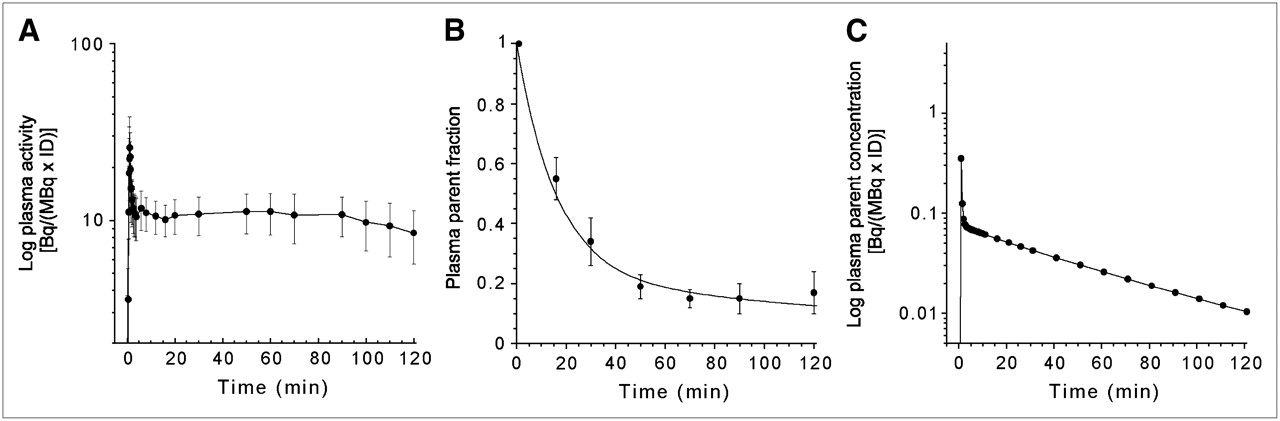
After an initial, rapid distribution phase, total plasma activity stabilized at a relatively constant level (Fig. 1A). 11C-DASB underwent significant metabolism over the duration of the study (Fig. 1B). At 30 min, 34% ± 8% of the total activity corresponded to the parent compound. The initial distribution volume (Vbol) of 11C-DASB was 40 ± 10 L. The estimated parent plasma input function (mean across 9 subjects) is shown in Figure 1C. The average parent plasma clearance rate was 163 ± 37 L·h−1; the clearance rate for the test condition was slightly lower than for the retest condition (146 ± 44 L·h−1 vs. 179 ± 36 L·h−1, P = 0.02). The test/retest variability for the clearance was 26% ± 18% with an ICC = 0.42. The free fraction of 11C-DASB in the plasma was 9.4% ± 1.5% and did not differ between conditions (n = 18, P = 0.89); test/retest variability = 13% ± 14%, ICC = 0.40.

(A) Mean ± SD of total plasma activity normalized to injected dose [Bq/(mL × MBq ID) after injection of 11C-DASB. Each point is mean of 9 subjects. After a rapid distribution, plasma activity stabilized to a relatively constant level. (B) Mean ± SD of fraction of plasma activity corresponding to parent compound after injection of 11C-DASB. Values are mean of 9 subjects. (C) Mean plasma activity corresponding to parent compound after injection of 11C-DASB. Each point is mean of 9 subjects.
Brain Analysis
Activity peaked relatively early in the cerebellum and neocortical regions (∼25 min) and later in the STR, MID, and THA (35–55 min) with intermediate values in the limbic regions (25–35 min). The degree of tracer washout, defined as the percentage decrease from the peak activity to the end of the scan, was high in most regions (37%–65%) with the exception of the SERT dense MID, where the washout was notably lower (16% ± 7%). The average ratios of ROI to cerebellar activity from 75 to 115 min were MID, 3.06 ± 0.45; THA, 2.26 ± 0.23; STR, 2.18 ± 0.21; MTL, 1.67 ± 0.19; ACC, 1.36 ± 0.16; and 1.25 ± 0.13, 1.13 ± 0.11, 1.12 ± 0.11, 1.09 ± 0.16, 1.08 ± 0.11 in the TC, OC, MPFC, OFC, and DLPFC, respectively.
1TC and 2TC Kinetic Analysis
The results from 1TC and 2TC analyses are shown in Tables 1 and 2, respectively. The 1TC model reached convergence for every study in all regions (n = 198). As stated earlier, an unconstrained 2TC model resulted in a high degree of nonconvergence. Only 22 of 198 regions converged (11%), with poor identifiability in most regions where convergence was obtained (identifiability < 10% in only 5 regions). Using the constrained 2TC model, convergence was achieved in all regions (n = 11) in each study (n = 18).
Reproducibility of 11C-DASB Total Distribution Volume (VT, mL·g−1), Binding Potential (BP, mL·g−1), and Specific-to-Nonspecific Equilibrium Partition Coefficient (V3″, Unitless) Derived via 1TC Kinetic Model
Reproducibility of 11C-DASB Total Distribution Volume (VT, mL·g−1), Binding Potential (BP, mL·g−1), and Specific-to-Nonspecific Equilibrium Partition Coefficient (V3″, Unitless) Derived via 2TC Kinetic Model
Cerebellum Distribution Volume.
Neither the 1TC nor the 2TC model demonstrated an advantage in goodness of fit for this region, as illustrated in Figure 2. The cerebellar VT calculated by the 1TC and 2TC were nearly identical. The VT identifiability was similar for both the 1TC (1.58% ± 0.44%) and the 2TC (2.37% ± 0.71%) models. The test/retest variability and reliability were also similar across methods, with VAR of <10% and ICC of >0.9 in all cases. Given the similarities between the 1TC and 2TC, neither model provided an improved cerebellar fit. Therefore, when determining the regional SERT receptor parameters by the 1TC or 2TC model, the same model used for the regional fit was used for the cerebellum fit.

Regional time–activity curves measured after injection of 551.3 MBq 11C-DASB in 33-y-old female. Regions displayed include MID (○), STR (□), MTL (⋄), MPFC (▵), and CER (▿). Points are measured activities in ROIs; lines are fitted values to 1TC model (solid line) and 2TC model (dashed line). Fits for both models are similar.
ROI Distribution Volumes.
As illustrated in Figure 2, the fits achieved in each ROI with either the 1TC or 2TC kinetic model were similar. Given this similarity, VT derived by either 1TC or 2TC analysis was nearly identical and highly correlated (r2 = 0.99, P < 0.0001, n = 180). The regional mean identifiability for VT was 1.69% ± 0.60% (n = 180; range, 1.39% ± 0.53% in THA to 2.33% ± 1.10% in MID) with the 1TC model and 2.27% ± 0.88% (n = 180; range, 1.54% ± 0.57% in THA to 2.88% ± 0.83% in the OFC) with the 2TC model. The variability of VT derived by either model was excellent. The average VAR in VT derived with the 1TC was 7.5% ± 0.9%; for the 2TC, the average VAR in VT was 7.4% ± 1.0%. The ICC values of VT for the 1TC and 2TC were excellent and identical at 0.93 ± 0.02.
SERT Parameter Analysis.
The 1TC and 2TC models provided similar estimates of BP as well as similar estimates of V3″ (Tables 1 and 2).
The reproducibility for the outcome measures BP and V3″ varied with regional SERT density. Tables 1 and 2 list the VAR and ICC for BP and V3″ across regions of high, moderate, and low SERT density for each method. For both BP and V3″, the test/retest variability increased as the SERT density of the region decreased. Overall, no difference in test/retest variability was observed between the methods for BP (RM ANOVA, P = 0.30) or V3″ (RM ANOVA, P = 0.22). Unlike the variability, the reliability did not vary by regional SERT density. The reliability of BP (1TC, 0.91 ± 0.06; 2TC, 0.91 ± 0.05) and V3″ (1TC, 0.87 ± 0.08; 2TC, 0.87 ± 0.09) was excellent across all regions.
Model Order Estimation.
The models were compared for goodness of fit by the F test (29,30) and AIC (28). The F test was significant (P < 0.05) in 51 of the 198 (9 subjects × 2 studies × 11 regions) fits examined, indicating that the higher-order model (2TC) provided a better fit for 26% of the datasets. The F test was generally significant on a study basis rather than a regional basis. In other terms, in 4 of the 18 studies, the 2TC provided a better fit than the 1TC in most regions, whereas, in the other studies, no benefit of the higher-order model was observed in the majority regions. The AIC of the 2TC model was lower than the AIC of the 1TC in 115 of the 198 fits examine (58%), indicating a better fit. The AIC and the F test shared the property that, across all regions, some studies were fitted better with a 2TC model than with the 1TC model. In all cases, when the F test indicated a better fit using the higher-order model (51/198), this was confirmed by the AIC.
DEPICT Analysis
The results from the DEPICT analysis are shown in Table 3.
Reproducibility of 11C-DASB Total Distribution Volume (VT, mL·g−1), Binding Potential (BP, mL·g−1), and Specific-to-Nonspecific Equilibrium Partition Coefficient (V3″, Unitless) Derived via DEPICT Analysis
Cerebellum Distribution Volume.
The DEPICT produced cerebellar VT nearly identical to the 1TC and 2TC estimates (RM ANOVA, P = 0.39). Similarly, the variability was excellent with a VAR of <10% and ICC of >0.9 in each case.
ROI Distribution Volumes.
Distribution volumes derived by DEPICT were highly correlated with the kinetic analysis (DEPICT = 1.00 × 2TC, r2 = 0.96, P < 0.0001). Significant differences were observed between DEPICT and both the 1TC and 2TC models (RM ANOVA, P < 0.0001). Post hoc analysis revealed that the VT derived with DEPICT was slightly, but significantly, lower than the 1TC or 2TC models only in the MID (e.g., 29.4 ± 7.2 mL·g−1 vs. 25.8 ± 4.8 mL·g−1, 2TC MID vs. DEPICT MID; Fisher's protected least-significant difference [PLSD] post hoc test, P = 0.0006). No differences were observed between DEPICT and the kinetic models in any other region.
The reproducibility of VT derived by DEPICT was similar to the 1TC and 2TC models, with a VAR of 7.8% ± 1.2% and ICC of 0.91 ± 0.02.
SERT Parameter Analysis.
The SERT parameters derived by DEPICT were highly correlated with the kinetic analysis (BP, DEPICT = 1.02 × 2TC, r2 = 0.95, P < 0.0001; V3,″, DEPICT = 1.03 × 2TC, r2 = 0.95, P < 0.0001). As with the VT, both BP and V3″ derived with DEPICT were significantly different than BP and V3″ derived with the 1TC and 2TC (RM ANOVA P < 0.0001 for both BP and V3″). Post hoc analysis revealed that BP and V3″ derived with DEPICT were slightly, but significantly, lower than the kinetic models only in the MID (e.g., BP, 19.9 ± 5.4 mL·g−1 vs. 16.3 ± 3.2 mL·g−1, 2TC MID vs. DEPICT MID; Fisher's PLSD, P = 0.0005). No differences were observed between DEPICT and the kinetic models in any other region. As with the kinetic models, the VAR for the outcome measures BP and V3″ derived via DEPICT increased as the SERT density of the region decreased. Overall, no difference in VAR was observed between DEPICT and the kinetic methods for BP (RM ANOVA, P = 0.43) or V3″ (RM ANOVA, P = 0.43). The ICC of BP (0.86 ± 0.05) and V3″ (0.82 ± 0.09), though still excellent, were slightly, but significantly, lower than those of the kinetic models (RM ANOVA, P < 0.0001 and P = 0.03, respectively).
Model Order Estimation.
The DEPICT plasma input method selected a 1TC model in 70 of the 198 fits, a 2TC model in 125 of the 198 fits, and a 3-tissue compartment (3TC) model in 3 of the 198 fits.
Graphical Analysis
The results from the graphical analysis are shown in Table 4.
Reproducibility of 11C-DASB Total Distribution Volume (VT, mL·g−1), Binding Potential (BP, mL·g−1), and Specific-to-Nonspecific Equilibrium Partition Coefficient (V3″, Unitless) Derived via Graphical Analysis
Cerebellum Distribution Volume.
The graphical analyses also produced cerebellar VT similar to the 1TC and 2TC estimates. The reproducibility of the cerebellar distribution volume derived with the graphical analysis was excellent, with a VAR of <10% and an ICC of >0.9 in each case.
ROI Distribution Volumes.
The regional total distribution volumes derived with the graphical method were highly correlated with those derived via both 1TC and 2TC models (r2 = 0.99, P = 0.0001, n = 198). Across regions, graphical VT values were 100.4% ± 2.5% those of the 1TC model and 101.3% ± 2.5% those of the 2TC model. The variability and ICC for the graphical VT data were similar to the kinetic models (variability, 8.3% ± 1.2%; ICC, 0.89 ± 0.03).
SERT Parameter Analysis.
As with VT, the regional values of BP and V3″ derived by the graphical method were highly correlated with those derived by either 1TC or 2TC model (for both models, BP and V3″: r2 = 0.99, P = 0.0001, n = 180). A significant difference was observed for V3″ derived via the 1TC and 2TC kinetic models compared with the graphical analysis (RM ANOVA, P < 0.001). Fisher PLSD post hoc analysis revealed significant differences (P < 0.05) in the high-binding regions (MID, THA, and STR), with the V3″ values in these regions derived via the graphical analysis being 1.5%–2.7% lower than those derived via the 1TC or 2TC models. No difference in VAR was observed between the graphical and kinetic methods for BP (RM ANOVA, P = 0.56) or for V3″ (RM ANOVA, P = 0.55). The ICC of BP (0.87 ± 0.08) and V3″ (0.84 ± 0.08) was lower than observed with the kinetic models (RM ANOVA, P = 0.0002 and P = 0.08, respectively).
SRTM Analysis
The results from the SRTM analyses are shown in Table 5. V3″ derived by the SRTM was highly correlated with plasma input based V3″ (e.g., SRTM [iterative] vs. 2TC, r2 = 0.99, P < 0.0001, n = 180). No difference in variability between the iterative method and the basis function method was seen (RM ANOVA, P = 0.30). The ICC observed with the iterative method was lower than that of the basis function method, although this did not reach the level of significance (iterative, 0.67 ± 0.26; basis, 0.81 ± 0.11, RM ANOVA, P = 0.15). A significant difference was observed in V3″ values derived via the 1TC and 2TC kinetic models compared with SRTM (RM ANOVA, P < 0.009). Fisher PLSD post hoc analysis revealed significant differences (P < 0.05) in the high-binding regions (MID, THA, and STR), with the V3″ values in these regions derived via SRTM being 5.8%–10.0% lower than those derived via the 1TC or 2TC model. Compared with the 1TC and 2TC models no difference was observed in the VAR measured for either SRTM method (RM ANOVA, P = 0.08). However, both SRTM analyses resulted in lower reliability than seen with the either the 1TC or 2TC models (RM ANOVA, P < 0.0001).
Reproducibility of 11C-DASB Specific-to-Nonspecific Equilibrium Partition Coefficient (V3″, Unitless) Derived via SRTM Analysis
Across Method Comparison of V3″
Table 6 provides the correlation between each of the 6 methods used to derived V3″ in this study. The r2 values listed in Table 6 are the square of the Pearson correlation coefficient determined between each method, for each subject, across all ROIs (n = 180). Excellent agreement existed across all methods, with the highest correlation seen between the 1TC, 2TC, and graphical methods.
Correlation of 11C-DASB V3″ Derived with Various Analytic Methods
DISCUSSION
The goal of this study was to evaluate the ability to accurately estimate regional SERT binding parameters with 11C-DASB PET by repeating each subject's PET scan on the same day and assessing reproducibility indices.
Outcome Measures and Models
Three outcome measures were examined in this study: the total distribution volume (VT), the binding potential (BP), and the specific-to-nonspecific partition coefficient (V3″). VT includes free and nonspecific as well as specific binding of the radiotracer so that its use as a direct outcome measure to infer binding properties should be restricted to situations where separate measurement of nonspecific binding is not possible (i.e., when no appropriate region of reference exists) and nonspecific binding is negligible relative to the specific binding (which is not the case for 11C-DASB). Its most frequent use is in situations such as the present study where a reference region does exist, so that BP and V3″ can be inferred indirectly in terms of VT from the ROI and the region of reference. BP does not include tissue nonspecific binding but is proportional to f1, the plasma free fraction, so that similar f1 values across populations is a prerequisite for comparisons using this parameter. V3″ is independent of f1 but is proportional to f2, the tissue free fraction, so that similar values of f2 across populations are necessary for making comparisons with this parameter.
A range of modeling techniques was used to estimate the outcome measures for this study. In this study the kinetic analysis was performed by 2 techniques (both using the arterial input function). The first technique assumed a specific compartment model, either 1TC or 2TC, to yield estimates of the rate constants governing transfer between the compartments, which were subsequently used to derive the outcome measures. The second, DEPICT, made no a priori assumption regarding the compartment model but, rather, derived the model order from the data (7). The second analytic method used to derive SERT binding parameters in this study was by use of reference region input with SRTM. SRTM is also a model-based method that uses a region of reference—in this case, the CER—as the input function for the model (6). This method restricts the outcome measure to V3″, with the attendant caveats regarding nonspecific binding. The final analytic method used in this study was graphical analysis (36), another data-driven method, in which a nonlinear transformation of the data leads to a linear relationship between the transformed variables, allowing determination of VT via linear regression.
In all, 14 outcome measures were evaluated: VT by 1TC, 2TC, DEPICT, and graphical methods; BP by 1TC, 2TC, DEPICT, and graphical methods; and V3″by a 1TC, 2TC, DEPICT, graphical, and SRTM, with the SRTM analyses performed by 2 approaches, iterative and basis function. Two criteria were assessed, the reliability and variability. Variability is the between-scan differences observed within subjects and reliability relates to the relative contributions of within- and between-subject variability—that is, the ability to detect true between-subject differences given the level of within-subject variability.
Comparison of DEPICT with Kinetic Methods
One goal of this study was to compare the results produced by DEPICT with those obtained with the 1TC and 2TC models. Using either a 1TC or 2TC model to derive VT, BP or V3″ gave nearly identical results for each outcome measure across all regions. The regional values of the outcome measures derived by the DEPICT method were similar to both the 1TC and 2TC models but slightly lower in the MID region. The MID is the region with the highest SERT density and, therefore, the highest VT. The DEPICT analysis resulted in a VT of 25.8 ± 4.8 mL·g−1in this region compared with 29.9 ± 7.6 mL·g−1 and 29.4 ± 7.3 mL·g−1 for the 1TC and 2TC models, respectively, with commensurately lower values of BP and V3″ in the MID, but nearly identical values for these outcome measures in other regions. The reason for this is that DEPICT is a basis function method and includes, as do most basis function implementations, truncation of the set of exponential rate constants associated with the basis function set at a finite positive number slightly larger than the theoretic lower limit (i.e., zero for decay-corrected data or the decay constant for uncorrected data). This is because, in the presence of statistical noise, identifiability of distribution volume estimates becomes poor near this limit. However, the approach may be associated with a small amount of bias at the highest distribution volumes. The tradeoff is a great increase in the stability of the estimates. This becomes particularly apparent in voxelwise analysis, as opposed to ROI analysis, where basis function methods perform well, but the decreased signal-to-noise level becomes prohibitively problematic for iterative methods. Also, given that both approaches used the same arterial input function data, the iterative methods do not necessarily represent a gold standard in this comparison. This issue needs to be further explored both through analysis of other datasets and by simulations in which “true” parameter values are known.
The VAR, of VT was excellent (<10%) in all regions, for both kinetic approaches and DEPICT. Similarly, in regions of high SERT density, the variability of BP and V3″ was also good (<10%). However, in regions of moderate and low SERT density, the variability associated with BP and V3″ was higher than that of VT. This is not unexpected, as BP and V3″ are derived via the difference in VT between the ROI and the region of reference, thereby increasing the effects of noise on the variability measurement. This is particularly evident when the VT in the ROI is close to V2, such as in the neocortical regions. In this study the variability of BP and V3″ derived by the kinetic methods ranged from 14.4% ± 1.6% to 17.2% ± 6.0% in the moderate-binding regions and was unacceptably high for all methods in the low-binding regions.
Unlike the variability, the reliability, as determined by the ICC, was less dependent on the regional SERT density. The ICC for VT was excellent (≈0.90) across all regions for the 1TC, 2TC, and DEPICT method. Similar values were observed for BP and V3″, indicating these methods should work equally well at discriminating differences at the group level.
Determination of Model Order
The question of determination of model order is typically posed in terms of a tradeoff between better goodness of fit achieved with a higher-order model and better robustness to noise achieved with a lower-order model. With the present dataset, 1TC and 2TC yielded very similar outcome measure estimates across all subjects and regions. The statistics designed to test model order, the F ratio and the Akaike score, were fairly split between models. On the datasets that these statistics identified the 1TC fit as more parsimonious, it might be expected that the VAR statistic would be better for the 1TC model, but this was not the case (RM ANOVA, P = 0.38). Thus, we can recommend the 2TC over the 1TC, based on the observation that the 2TC fit is better for some datasets but there is no apparent loss of stability with 2TC compared with 1TC. In the context of this dataset, it was particularly interesting to examine the behavior of DEPICT. DEPICT is a method designed to estimate model order automatically and it was fairly split between 1TC and 2TC as well (a small number of fits were designated 3TC). The F ratio and Akaike score from the 1TC and 2TC models were not well correlated with DEPICT. For example, the mean F value from the regions designated 1TC by DEPICT was slightly but significantly higher than in those designated 2TC, with similar results for Akaike. The impulse response fraction is another parameter related to model order (37) that measures the fraction of the total area under the curve resulting from the convolution of the input function with the faster of the 2 exponential functions in the response function of a 2TC model. It has been conjectured that very small impulse response fraction is associated with poor identifiability of 2 distinct compartments in a brain region. The impulse response fraction from the 2TC fits in the present dataset bear an intriguing relationship to model order as determined by DEPICT (Fig. 3). When the impulse response fraction is <0.01, the DEPICT model order is spread between 1TC and 2TC with all 4 3TC fits falling into this range as well. However, for 24 of the 29 fits for which the impulse response fraction is >0.005 and 13 of the 13 fits where the impulse response fraction is >0.01, the DEPICT model order estimate was 2. It remains for future work to further explore this relationship, particularly with ligands for which the impulse response fraction is more heterogeneous.

Relationship between impulse response fraction (IRF) generated from kinetic 2TC data and model order chosen by DEPICT. In the case when the IRF is small (<0.005, below dashed horizontal line), model order is spread between 1TC and 2TC without clear bias toward one or the other. However, for IRF of >0.005, the DEPICT method settled nearly exclusively on the 2TC model. This is particularly evident for IRF of >0.01 (above solid horizontal line).
Evaluation of Graphical Analysis
Distribution volumes derived by graphical analysis were strongly correlated with VT derived by both the 1TC and 2TC models (r2 = 0.99, P = 0.0001, n = 180), with similar values of VT (99.2% ± 2.5%), excellent test/retest variability (< 10%) and ICC (≈ 0.90). Unlike Ginovart et al., we did not find study-wide reduction in the values of VT derived with the graphical analysis when compared with the kinetic analysis (2). We have reported a tendency for this method to underestimate VT values in the past (38), but this is a statistical property, rather than a systematic property, of the method and was not evident in the present dataset. As with the kinetic analyses, the variability for the outcome measures BP and V3″ with the graphical analysis was similar to VT in the high-binding regions (10.6% ± 4.3%) and lower in the limbic (18.4% ± 7.1%) and neocortical (41.7% ± 11.1%) regions. The ICC of both BP and V3″ for the graphical analysis was good across all regions (> 0.75).
Evaluation of SRTM
SRTM provided values of V3″ that, in most regions, were similar to those achieved with the 1TC and 2TC models. However in MID, both the iterative and basis function approach produced lower estimates by 10%−15% compared with the 1TC and 2TC, as observed in a previous study (2). In addition, the reliability of the iterative implementation was noticeably lower than other methods, including basis function SRTM, particularly in the moderate and low-binding regions. Also, though no method had acceptable reliability in the low-binding regions, the iterative SRTM produced V3″ estimates in low-binding regions that were clearly out of line with all other methods in select cases, although the average values remained similar, and was associated with unacceptably poor identifiability in these regions. It is not unexpected for basis function implementations to be more robust in high-noise situations (39), but the present study lends emphasis to the observation that basis function implementations are more stable when low signal-to-noise ratio derives not just from random error but from situations where specific binding comprises a small fraction of the signal.
CONCLUSION
The results of this study indicate that 11C-DASB can be used to measure SERT parameters with high reproducibility in receptor-rich, central regions of the brain, with somewhat less, yet still acceptable, reproducibility in regions of moderate SERT density and poor reproducibility in low-density regions. No clear advantage was evident in the choice of analytic methods, as all methods examined gave similar values across all regions. Therefore, the choice of methods is dependent on the experimental situation, with some caveats. Examination of the 1TC and 2TC fits indicates that the higher-order model may provide a better fit in some studies. Alternatively, the DEPICT method offers a convolution algorithm approach that makes no a priori assumptions regarding model order, albeit with a small amount of bias in the highest binding regions induced by the truncation of the basis set away from the slowest washout rates. In the absence of an arterial input function, SRTM provides an alternative method of analysis, subject to the limitations imposed by the possibility of different levels of nonspecific binding across populations (40). Finally, the basis function implementation of SRTM provides better reliability than the iterative version of this method, particularly in low- and moderate-binding regions, subject again to a small amount of bias in the highest binding regions.
Acknowledgments
This work was supported in part by grants from NARSAD, NIMH (1 R21 MH66624-01, 1K08 MH 069697-01A1, 1-K02-MH01603-01, 5 P50 MH066171-02), and the Lieber Center for Schizophrenia Research at Columbia University. The authors thank Alan Wilson for providing the precursor for 11C-DASB and acknowledge the technical assistance of Julie Arcement, Jennifer Bae, Susan Curry, Ingrid Gelbard-Strokes, Charisse Green, Elizabeth Hackett, Kimchung Ngo, Chaka Peters, Nurat Quadri, Celeste Reinking, Norman Simpson, Lyudmila Savenkova, Kris Wolff, and Zohar Zephrani.
References
- Received for publication September 26, 2005.
- Accepted for publication January 11, 2006.


Jump to section
Related Articles
Cited By...
- Preserved Serotonin Transporter Availability in Parkinson Disease Measured with Either [11C]MADAM or [11C]DASB: A Study Including 2 Separate Cohorts of Nondepressed Patients
- Test-Retest Reliability of the SERT Imaging Agent 11C-HOMADAM in Healthy Humans
- In Vivo Evaluation of 11C-DASB for Quantitative SERT Imaging in Rats and Mice
- Monoamine Transporter Occupancy of a Novel Triple Reuptake Inhibitor in Baboons and Humans Using Positron Emission Tomography
- Serotonin Transporters in Dopamine Transporter Imaging: A Head-to-Head Comparison of Dopamine Transporter SPECT Radioligands 123I-FP-CIT and 123I-PE2I
- Human 5-HT Transporter Availability Predicts Amygdala Reactivity In Vivo
- Test Retest Reproducibility of 18F-MPPF PET in Healthy Humans: A Reliability Study