HOME HELP FEEDBACK SUBSCRIPTIONS ARCHIVE SEARCH TABLE OF CONTENTS		QUICK SEARCH:   [advanced] Author: Keyword(s): Year:  Vol:  Page:

This Article Abstract Figures Only Full Text (PDF) Alert me when this article is cited Alert me if a correction is posted Services Email this article to a friend Similar articles in this journal Similar articles in PubMed Alert me to new issues of the journal Download to citation manager Citing Articles Citing Articles via HighWire Citing Articles via Google Scholar Google Scholar Articles by Vanhove, C. Articles by Bossuyt, A. Search for Related Content PubMed PubMed Citation Articles by Vanhove, C. Articles by Bossuyt, A.

Automatic Determination of Left Ventricular Ejection Fraction from Gated Blood-Pool Tomography

Division of Nuclear Medicine, University Hospital, Free University of Brussels, Brussels, Belgium

	ABSTRACT

TOP ABSTRACT INTRODUCTION MATERIALS AND METHODS RESULTS DISCUSSION CONCLUSION REFERENCES

 
The aim of this study was to develop and validate a new algorithm to automatically compute left ventricular ejection fraction (LVEF) from gated blood-pool tomography (GBPT). The results were compared with those of conventional planar radionuclide angiocardiography (PRNA). Methods: Fifty-three consecutive patients received an injection of 740 MBq ^99mTc-labeled human serum albumin. PRNA and GBPT were performed consecutively in a random sequence. PRNA served as the reference, and GBPT images were processed using a new edge detection algorithm. The algorithm is fast (<45 s), fully automatic, and works in three-dimensional space. The method includes identification of the valve plane and the septum. The left ventricular cavity at end-diastole is delineated by segmentation using an iterative threshold technique. An optimal threshold is reached when the corresponding isocontour best fits the first derivative of the end-diastolic count distribution in three dimensions. This optimal threshold is then applied to delineate the left ventricular cavity on the other time bins. The data are corrected for the partial-volume effect. Left ventricular volumes are determined using a geometry-based method and are used to calculate the ejection fraction. Results: The success rate of the new algorithm was 94%. LVEFs calculated from GBPT agreed well with those calculated from PRNA (r = 0.78; GBPT = 0.94 PRNA + 6.33). The systematic error was 2.8%, and the random error was 8.8%. Excellent inter- and intraobserver reproducibility was found, with average differences of 1.1% ± 4.6% and 1.1% ± 5.0%, respectively, between the two measurements. Conclusion: This new algorithm provides a fast, automated, and objective method to calculate LVEF from GBPT.

Key Words: blood-pool SPECT • automatic algorithm • left ventricular ejection fraction

	INTRODUCTION

TOP ABSTRACT INTRODUCTION MATERIALS AND METHODS RESULTS DISCUSSION CONCLUSION REFERENCES

 
Gated blood-pool tomography (GBPT) is the three-dimensional analog of standard planar radionuclide angiocardiography (PRNA). The rationale for the use of GBPT is that left ventricular function can be determined more accurately because the overlap of the cardiac chambers can be avoided. The need for background subtraction, which is a requirement for planar gated blood-pool imaging, is also eliminated. Furthermore, the three-dimensional nature of the tomographic data lends itself naturally to a space-based rather than count-based analysis when geometric assumptions for volume estimation are needed.

In contrast to the widespread use of gated SPECT in myocardial perfusion scintigraphy (1), GBPT has not yet become routine for cardiac gated blood-pool studies. The small dimensions of the myocardial wall compared with the volume of left ventricular blood causes partial-volume effects in gated myocardial perfusion tomography; this error is less of a problem in GBPT. Consequently, cardiac volumes can be estimated more accurately with GBPT than with gated myocardial perfusion tomography. Moreover, the number of cardiac counts collected per millicurie of injected radioactivity is higher for GBPT (2), and the separation between left and right ventricles conceptually allows blood-pool studies to measure right ventricular function.

Despite these advantages, GBPT has not yet become widely used because of the lack of automatic, fast, and reliable quantitative algorithms for measuring ventricular ejection fraction from GBPT. Threshold methods, count-based methods, and local gradient methods have been proposed (3–16). In the threshold method, voxels higher than a predetermined threshold are included as part of the cardiac volume. This threshold is usually determined from phantom studies. In the count-based method, the total volume of the cavity is derived from the number of counts measured within a small volume of interest of known dimensions. In the local gradient method, the edge of the cavity volume is detected using the first and second derivatives along count density profiles. Most of these methods require a degree of manual operation for masking, setting threshold values, and setting limits for a boundary search.

The aim of this study was to develop and validate a new algorithm to calculate left ventricular ejection fraction (LVEF) from GBPT. In this algorithm, an automatic three-dimensional segmentation technique was applied, combining the threshold and the local gradient methods, to delineate the left ventricular cavity. The results were compared with those of PRNA.

	MATERIALS AND METHODS

TOP ABSTRACT INTRODUCTION MATERIALS AND METHODS RESULTS DISCUSSION CONCLUSION REFERENCES

 
Patient Population
The population consisted of 53 consecutive patients (23 men, 30 women; age range, 23–83 y; mean age, 63 y) referred to the Division of Nuclear Medicine for evaluation of left ventricular function with radionuclide angiocardiography. Sixteen patients had a history of acute myocardial infarction, and 37 patients were receiving chemotherapy. All patients received a 740-MBq injection of ^99mTc-labeled human serum albumin (HSA). Planar radionuclide angiocardiograms and gated blood-pool tomograms were acquired consecutively in a random sequence after informed consent was given.

PRNA
PRNA was performed using 16 electrocardiographic gated frames, forward–backward framing, and a beat acceptance window at 20% of the average R-R interval obtained just before starting acquisition of a left anterior oblique projection (best septal view). The projection was acquired using one head of a triple-head gamma camera (MultiSPECT3; Siemens, Hoffman Estates, IL) equipped with a low-energy, high-resolution collimator. Data were acquired in 64 x 64 format with a zoom of 2.29 (pixel size, 3.1 mm) until a total density of 4 million counts was reached.

For determination of LVEF, the images were transferred onto an NXT (P) computer (Sopha Medical Vision, Paris, France) and processed with a commercially available fully automatic program, Gated Equilibrium Bloodpool Processing, version 2.0.

GBPT
The GBPT studies were acquired with a MultiSPECT3 gamma camera equipped with low-energy, high-resolution collimators. Parameters of acquisition were as follows: 360° stop-and-shoot rotation, 32 stops per head (96 projections), 30 s per stop, 64 x 64 matrix, zoom of 1.23 (5.79-mm pixel size), eight time bins using 75% forward–backward framing, and a beat acceptance window at 20% of the average R-R interval calculated just before starting the acquisition.

The projection data were reconstructed by filtered backprojection applying a Butterworth filter with a cutoff frequency of 0.35 cycles per centimeter and an order of 5. The reconstructed slices were reoriented according to the left ventricular long axis. The gated horizontal long-axis slices were used as input for the new algorithm.

The New Algorithm
The new algorithm uses geometric methods to delineate the left ventricular cavity, is fully automatic, and works in three-dimensional space. The execution time is approximately 45 s on a Macintosh G3 computer (Apple Computer, Inc., Cupertino, CA). It comprises the following steps: detection of the valve plane, detection of the interventricular septum, delineation of the left ventricular cavity at end-diastole, delineation of the left ventricular cavity for the other time bins, and calculation of left ventricular volumes and ejection fraction.

Detection of Valve Plane.
Automatic detection of the valve plane is important for separating the ventricles from the atria. The three-dimensional image at end-systole was subtracted from the end-diastolic image to detect the valve plane. End-diastole was defined as the first time bin. End-systole was defined as the time bin in which the absolute difference with respect to the end-diastolic frame was maximal. Only voxels with a count density greater than 50% of the maximum count density found at end-diastole were considered. In the subtraction image, the voxels at the borders of the ventricles become positive, whereas the voxels close to the atria turn out to be negative (Fig. 1). The valve plane was defined as the collection of voxels that satisfy the following condition:

(Eq. 1)

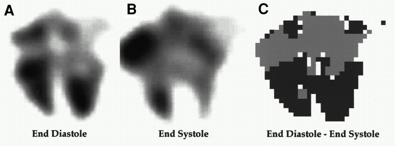
View larger version (43K): [in this window] [in a new window]   FIGURE 1. Horizontal long-axis slice at end-diastole (A) and end-systole (B). Subtracting end-systolic image from end-diastolic image (C) results in positive values around ventricles (dark gray) and negative values around auricles (light gray).

(Eq. 2)

This factor F was calculated using all voxels identified by their coordinates x, y, and z. p_xyz⁺ and p_xyz^- represent the number of voxels with positive values positioned in front of or behind the valve plane, respectively. In contrast, n_xyz^- and n_xyz⁺ are the number of voxels with negative values located behind and in front of the valve plane, respectively. Once F was maximized, voxels in front of the valve plane were identified as ventricular, whereas voxels behind the valve plane were recognized as auricular. Voxels behind the valve plane were not considered for further processing.

Detection of Interventricular Septum.
The septum was detected so that the right ventricle could be separated from the left ventricle. All short-axis slices at end-diastole containing voxels that were on the ventricular side of the valve plane were summed to obtain a two-dimensional best-septal-view image of the left and right ventricles. Again, only voxels with a count density greater than 50% of the maximum count density found at end-diastole were considered.

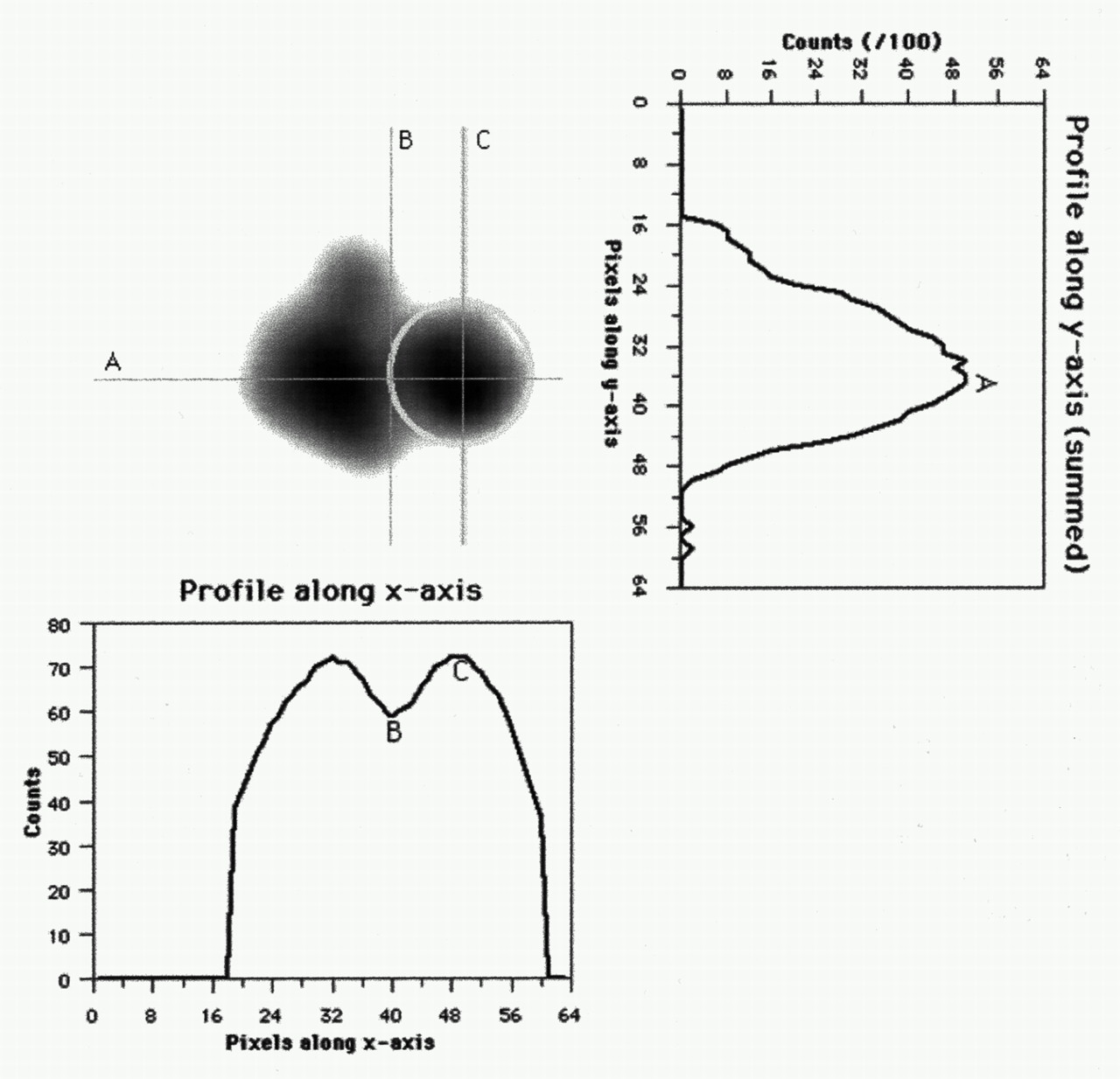
By summing, in this two-dimensional image, all pixels along the x-axis, a one-dimensional profile was generated (Fig. 2). The position of the local maximum (point A) in this profile was selected as the most likely location for the center of both ventricles. A profile along this position was created, and the local minimum was selected as the position of the septum (point B). The local maximum positioned on the left cardiac side of this local minimum was selected as the center of the left ventricle (point C).

View larger version (51K): [in this window] [in a new window]   FIGURE 2. Detecting septum is done on best septal view at end-diastole. By summing all voxels along x-axis, profile is generated. Maximum (A) is selected, and another profile along this location is created. Local minimum (B) is selected as septum, and local maximum on left side of septum (C) is selected as center of left ventricle.

Delineation of Left Ventricular Cavity at End-Diastole.
The segmentation started by applying a 30% threshold to the end-diastolic time bin. Only voxels having count densities higher than this threshold were considered.

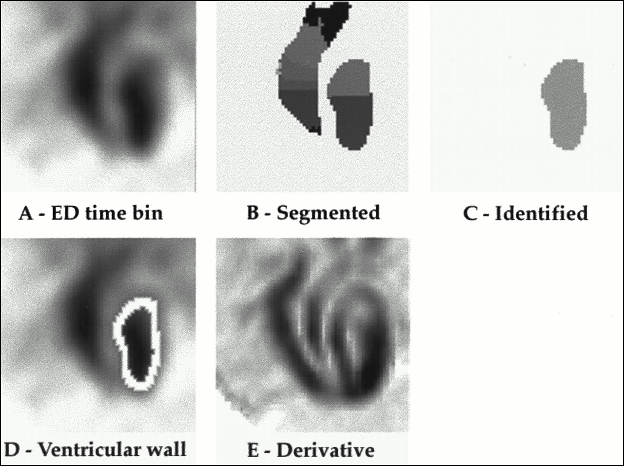
First, all local maximums in the image were detected, that is, all voxels that had higher count densities than their 26 neighbors in the three-dimensional image space. These voxels were called roots. All roots were labeled with a unique index. Voxels that were not labeled as roots were linked to a root by reaching it using the steepest slope path. The steepest slope path was defined as the collection of voxels having the largest difference from one of its 26 neighbors. All voxels reaching the same root were labeled with the index of that root. Figures 3A and B show, respectively, an original and a segmented end-diastolic horizontal long-axis slice. Finally, segments with roots on the ventricular side of the valve plane and on the left side of the detected septum were identified as the left ventricle (Fig. 3C).

View larger version (88K): [in this window] [in a new window]   FIGURE 3. Summary of algorithm. Initially, end-diastolic image (A) is segmented (B) and segments are identified (C) as left and right ventricle. Optimal threshold is found when corresponding ventricular wall (D) best fits first derivative of end-diastolic count distribution (E).

(Eq. 3)

where c_xyz represents the count density of voxel v at location (x, y, z) and c_ijk corresponds to the count densities of the 26 neighbors of voxel v. d_{xyz - ijk} is the distance between location (x, y, z) and location (i, j, k). An example is displayed in Figure 3E.

Delineation of Left Ventricular Cavity for Other Time Bins.
The delineation of the left ventricular cavity in the remaining time bins was done using the segmentation procedure and applying the threshold optimized for the end-diastolic delineation and corrected for a possible partial-volume effect. Accurate measurement of smaller ventricular volumes during the cardiac cycle can become difficult because of the limited resolution of the gamma camera, which leads to a partial-volume effect and results in an overestimation of the smaller volumes (8). To overcome this problem, the threshold initially applied was increased to compensate for the influence on the smaller volumes. The following formula was used to relate the loss of peak count density to the threshold required:

(Eq. 4)

T_ED and T_Corr represent the thresholds applied at end-diastole and after correction for a possible partial-volume effect, respectively. P_ED is the loss of peak count density, at a specific time bin, proportional to end-diastole and expressed as a percentage. This expression was derived after measuring a series of ^99mTc-filled spheres of known volumes. After the segmentation of a specific time bin, segments with roots within the left ventricle delineated at end-diastole were identified as the left ventricle for that time bin.

Calculation of Left Ventricular Volumes and Ejection Fraction.
Once the left ventricle was delineated for each time bin, the volumes of the cavity were calculated by summing all voxels. To provide continuity to the measured volumes during the cardiac cycle, a temporal fit based on a Fourier series, keeping only the first two harmonics, was applied to the calculated volumes. End-diastolic volume (EDV) and end-systolic volume (ESV) were defined as the largest and smallest volumes, respectively, on the fitted volume–time curve. Ejection fraction was computed as (EDV - ESV)/EDV and expressed as a percentage.

Inter- and Intraobserver Reproducibility
The inter- and intraobserver reproducibility of the new algorithm, used to calculate LVEF from GBPT studies, was determined as usual. Interobserver reproducibility was determined by processing the GBPT studies two times by two observers. Intraobserver reproducibility was determined by processing the GBPT studies two times by the same observer at a 3-mo interval.

Effect of Reconstruction Filter
The effect of the reconstruction filter on the LVEF measured from GBPT was evaluated on 20 randomly selected studies reconstructed using a Butterworth filter with cutoff frequencies of 0.25, 0.30, 0.35, 0.40, and 0.45 cycles per centimeter. Each dataset was then reoriented with the same angles to eliminate variability caused by reorientation.

Statistical Analysis
Linear regression analysis was used to compare the calculated LVEFs. Slope, intercept, and correlation coefficient were calculated. The Bland-Altman method (17) was used to calculate the systematic and random errors between GBPT and PRNA. Differences between the repeated measurements were evaluated by the paired Student t test, and P < 0.05 was considered significant.

	RESULTS

TOP ABSTRACT INTRODUCTION MATERIALS AND METHODS RESULTS DISCUSSION CONCLUSION REFERENCES

 
Success Rate
Among the 53 gated blood-pool tomograms, three datasets were incorrectly delineated, resulting in a success rate of 94% for the new algorithm. Failures were identified by visual inspection of the regions of interest delineating the left ventricle in the three dimensions and for each time bin. Errors in determining the valve plane were observed for two patients, and errors in delineating the interventricular septum were observed for one patient.

GBPT Versus PRNA
Figure 4A shows the relationship between LVEF measured with GBPT and LVEF measured with PRNA for the 50 patients with adequate delineation of the left ventricular cavity. The correlation coefficient between the two methods was 0.78 (slope = 0.94; intercept = 6.33). The mean difference (systematic error) between the GBPT and PRNA was +2.8%, with an SD (random error) of 8.8%. The t statistics indicated a P of 0.03, with mean values for the ejection fraction of 58% ± 14% and 55% ± 11% for GBPT and PRNA, respectively.

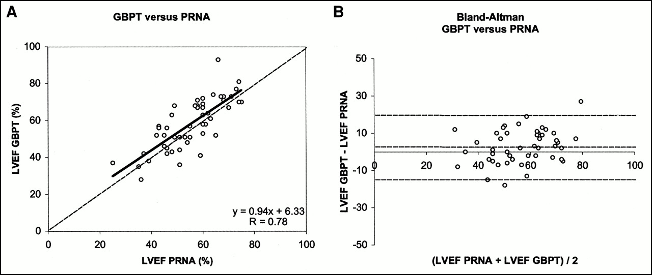
View larger version (15K): [in this window] [in a new window]   FIGURE 4. Linear regression analysis (A) and Bland-Altman plot (B) between LVEF determined by GBPT and LVEF determined by PRNA.

Intraobserver Reproducibility
Figure 5 shows the intraobserver reproducibility of the measured LVEF from GBPT. An excellent correlation between both measurements was observed (r = 0.94; slope = 0.91; intercept = 6.41). The systematic error was +1.1%, and the random error was 4.6%. No significant difference was observed between either series of measurements.

View larger version (14K): [in this window] [in a new window]   FIGURE 5. Intraobserver reproducibility. Linear regression (A) and Bland-Altman analysis (B) between original LVEFs measured (LVEF 1) and ejection fraction measured 3 mo later (LVEF 2).

View larger version (14K): [in this window] [in a new window]   FIGURE 6. Agreement between LVEFs measured by two independent observers.

	DISCUSSION

TOP ABSTRACT INTRODUCTION MATERIALS AND METHODS RESULTS DISCUSSION CONCLUSION REFERENCES

 
Gated cardiac blood-pool tomography has the intrinsic ability to accurately measure LVEF because the overlap between the left ventricle and the surrounding cardiac chambers is eliminated and background correction is not necessary. Moreover, the three-dimensional nature of GBPT lends itself naturally to a space-based rather than count-based analysis in which geometric assumptions for volume estimation are needed. In addition, GBPT has the potential to yield more accurate regional wall motion analysis and to investigate the right ventricle. Despite these advantages, its widespread use has been hampered by the unavailability of automatic, fast, and reliable algorithms to measure LVEF.

In this article, a new, fully automatic algorithm to compute LVEF from GBPT is presented. The new algorithm applies a three-dimensional segmentation technique combining threshold and local gradient methods to delineate the left ventricular cavity. The new algorithm is fast, has a high success rate, agrees well with conventional PRNA, and is reproducible.

The success rate of the algorithm was 94% among the 53 consecutive patients included in this study. The algorithm failed to correctly detect the left ventricular valve plane in two GBPT studies with poor count statistics, resulting in noisy images. The noise was further amplified when the end-diastolic and end-systolic images were subtracted. Left ventricular count density measured on the best-septal-view projection after summing all time frames was approximately 80 counts per pixel for these two patients, compared with 239 ± 62 counts per pixel for patients with adequate delineation of the valve plane. We therefore recommend that gated blood-pool studies contain at least 100 counts per pixel in the left ventricle. This goal can be achieved by increasing the dose in obese patients or, preferably, by adapting the time per stop after performing a short static acquisition in the best septal view just before starting the GBPT study.

Errors in locating the interventricular septum were observed for one patient with a very large left ventricle but a normal right ventricle. In this patient, the two ventricles merged into one and the algorithm was unable to separate them. Caution is therefore recommended when using this algorithm in patients with severe dilated cardiomyopathies involving either the left or the right ventricle.

LVEFs calculated on GBPT, although providing slightly higher values on average, agreed well with LVEFs calculated on PRNA. Although PRNA is probably not the ideal gold standard for measuring LVEF, this technique is still the most objective, reproducible, and widely used to measure LVEF in humans. That the correlation coefficient between the two techniques was only fair was not surprising, because PRNA is a planar imaging technique whereas GBPT is tomographic. The overlap between the left ventricle and the surrounding cardiac chambers (principally the left atrium) is eliminated with GBPT, and background correction is not necessary. Interestingly, the two methods compared better in patients with an LVEF less than 50% than in patients with an LVEF greater than 50%. No significant difference was seen between LVEF measured with GBPT and LVEF measured with PRNA in patients with an LVEF less than 50%. In contrast, LVEF measured with GBPT was significantly higher in patients with an LVEF greater than 50%. Higher LVEFs by GBPT than by PRNA have also been reported recently for studies by Mariano-Goulart et al. (15) and Van Kriekinge et al. (16).

In gated studies, counts have to be distributed over several time frames. For a given injected dose and acquisition time, the shorter the number of intervals the better the statistical quality of the individual time frames. Therefore, eight frames per cardiac cycle are usually preferred in gated SPECT. LVEFs measured with eight frames are, on average, 4% lower than 16-frame gated SPECT (1). This decrease is constant over a wide range of LVEFs. In this study, the predictable underestimation of LVEF was reduced by temporally fitting the calculated left ventricular volume curve during the cardiac cycle using the first two harmonics of the Fourier transform. LVEF was calculated using the maximum (EDV) and minimum (ESV) of the fitted curve.

The new algorithm is robust and reproducible. Because the algorithm is fully automatic, intra- and interobserver variability in measuring LVEF from GBPT occurred because of small variations in the reorientation of the reconstructed transverse tomograms along the long axis of the left ventricular cavity. However, the three-dimensional nature of the new algorithm minimizes this potential source of variability, as was confirmed by the excellent intra- and interobserver reproducibility. Importantly, the algorithm was also found to be little influenced by the reconstruction filter.

	CONCLUSION

TOP ABSTRACT INTRODUCTION MATERIALS AND METHODS RESULTS DISCUSSION CONCLUSION REFERENCES

 
A new algorithm has been presented to automatically compute LVEF from GBPT. The algorithm is fast, has a high success rate, agrees well with conventional PRNA, and is reproducible. Further evaluation of its accuracy requires phantom studies and comparison with other imaging modalities in patients. The algorithm also allows automatic delineation of the right ventricular cavity but has not been validated.

	FOOTNOTES

 
Received May 19, 2000; revision accepted Sep. 29, 2000.

For correspondence or reprints contact: Christian Vanhove, MSc, Division of Nuclear Medicine, University Hospital, Free University of Brussels (AZ VUB), 101 Laarbeeklaan, B-1090 Brussels, Belgium.

	REFERENCES

TOP ABSTRACT INTRODUCTION MATERIALS AND METHODS RESULTS DISCUSSION CONCLUSION REFERENCES

 

1. Germano G, Kiat H, Kavanagh PB, et al. Automatic quantification of ejection fraction from gated myocardial perfusion SPECT. J Nucl Med 1995;36:2138–2147.[Abstract/Free Full Text]
2. Germano G, Van Kriekinge S. Quantitative gated blood pool SPECT. In: Germano G, Berman DS, eds. Clinical Gated Cardiac SPECT Armonk, NY: Futura Publishing; 1999:339–347.
3. Underwoord SR, Walton S, Ell PJ, et al. Gated blood-pool emission tomography: a new technique for the investigation of cardiac structure and function. Eur J Nucl Med 1985;10:332–337.[Medline]
4. Corbett JR, Jansen DE, Lewis SE, et al. Tomographic gated blood pool radionuclide ventriculography: analysis of wall motion and left ventricular volumes in patients with coronary artery disease. J Am Coll Cardiol. 1985;6:349–358.[Abstract]
5. Bunker SR, Hartshorne MF, Schmidt WP, et al. Left ventricular volume determination from single-photon emission computed tomography. AJR. 1985;144:295–298.[Abstract/Free Full Text]
6. Caputo GR, Graham M, Brust KD, Kennedy JW, Nelp WB. Measurement of left ventricular volume using single-photon emission computed tomography. Am J Cardiol. 1985;56:781–786.[Medline]
7. Bingham J, Okada R, McKusick K, et al. Comparison of three semiautomatic methods for determination of left ventricular ejection fraction from gated cardiac blood pool images. Eur J Nucl Med. 1985;10:494–499.[Medline]
8. Mortelmans L, Nuyts J, Van Pamel G, Van den Maegdenbergh V, De Roo M, Suetens P. A new thresholding method for volume determination by SPECT. Eur J Nucl Med. 1986;12:284–290.[Medline]
9. Faber TL, Corbett JR. Acquisition and processing of tomographic radionuclide ventriculograms. In: Reiber JHC, van der Wall EE, eds. Cardiovascular Nuclear Medicine and MRI. Dordrecht, The Netherlands: Kluwer; 1992:181–191.
10. Ekman M, Lomsky M, Stromblad SO, Carlsson S. Closed-line integral optimization edge detection algorithm and its application in equilibrium radionuclide angiocardiography. J Nucl Med. 1995;36:1014–1018.[Abstract/Free Full Text]
11. Nelson AD, Muswick GJ, Muzic RF Jr, Deschamps X. A robust edge detection method for gated radionuclide ventriculograms. J Nucl Med. 1996;37:685–689.[Abstract/Free Full Text]
12. Barlett ML, Srinivasan G, Barker WC, Kitsiou AN, Disizian V, Bacharach SL. Left ventricular ejection fraction: comparison of results from planar and SPECT gated blood-pool studies. J Nucl Med. 1996;37:1795–1799.[Abstract/Free Full Text]
13. McKiddie FI, Gemmell HG, Redpath TW, et al. A variable threshold edge-detector for improved quantification of gated tomographic imaging of the left ventricular blood pool. Nucl Med Commun. 1996;17:410–417.[Medline]
14. Chin BB, Bloomgarden DC, Xia W, et al. Right and left ventricular volume and ejection fraction by tomographic gated blood-pool scintigraphy. J Nucl Med. 1997;38:942–948.[Abstract/Free Full Text]
15. Mariano-Goulart D, Collet H, Kotzki PO, Zanca M, Rossi M. Semi-automatic segmentation of gated blood pool emission tomographic images by watersheds: application to the determination of right and left ejection fractions. Eur J Nucl Med. 1998;25:1300–1307.[Medline]
16. Van Kriekinge SD, Berman DS, Germano G. Automatic quantification of left ventricular ejection fraction from gated blood pool SPECT. J Nucl Cardiol. 1999;6:498–506.[Medline]
17. Bland JM, Altman DG. Statistical methods for assessing agreement between two methods of clinical measurement. Lancet. 1986;1:307–310.[Medline]

This article has been cited by other articles:

				D. Mariano-Goulart, L. Dechaux, F. Rouzet, E. Barbotte, C. Caderas de Kerleau, M. Rossi, and D. Le Guludec Diagnosis of Diffuse and Localized Arrhythmogenic Right Ventricular Dysplasia by Gated Blood-Pool SPECT J. Nucl. Med., September 1, 2007; 48(9): 1416 - 1423. [Abstract] [Full Text] [PDF]

				P. De Bondt, T. Claessens, B. Rys, O. De Winter, S. Vandenberghe, P. Segers, P. Verdonck, and R. A. Dierckx Accuracy of 4 Different Algorithms for the Analysis of Tomographic Radionuclide Ventriculography Using a Physical, Dynamic 4-Chamber Cardiac Phantom J. Nucl. Med., January 1, 2005; 46(1): 165 - 171. [Abstract] [Full Text] [PDF]

				P. De Bondt, K. Nichols, S. Vandenberghe, P. Segers, O. De Winter, C. Van de Wiele, P. Verdonck, A. Shazad, A. H. Shoyeb, and J. De Sutter Validation of Gated Blood-Pool SPECT Cardiac Measurements Tested Using a Biventricular Dynamic Physical Phantom J. Nucl. Med., June 1, 2003; 44(6): 967 - 972. [Abstract] [Full Text] [PDF]

				G. A. Wright, S. Thackray, S. Howey, and J. G. Cleland Left Ventricular Ejection Fraction and Volumes from Gated Blood-Pool SPECT: Comparison with Planar Gated Blood-Pool Imaging and Assessment of Repeatability in Patients with Heart Failure J. Nucl. Med., April 1, 2003; 44(4): 494 - 498. [Abstract] [Full Text] [PDF]

				H. Okazawa, M. Takahashi, T. Hata, K. Sugimoto, Y. Kishibe, and T. Tsuji Quantitative Evaluation of Myocardial Blood Flow and Ejection Fraction with a Single Dose of 13NH3 and Gated PET J. Nucl. Med., August 1, 2002; 43(8): 999 - 1005. [Abstract] [Full Text] [PDF]

This Article Abstract Figures Only Full Text (PDF) Alert me when this article is cited Alert me if a correction is posted Services Email this article to a friend Similar articles in this journal Similar articles in PubMed Alert me to new issues of the journal Download to citation manager Citing Articles Citing Articles via HighWire Citing Articles via Google Scholar Google Scholar Articles by Vanhove, C. Articles by Bossuyt, A. Search for Related Content PubMed PubMed Citation Articles by Vanhove, C. Articles by Bossuyt, A.