


Abstract
Quantitative brain 18F-FDG PET studies often require the plasma time–activity curve (input function) for estimation of the cerebral metabolic rate of glucose (CMRglc). The gold standard for input function measurement is arterial blood sampling, which is invasive and time-consuming. Alternatively, input function can be estimated from dynamic images. This estimation often implies the use of manually placed regions of interest (ROIs) over cerebral vasculature, which is an operator-dependent and time-consuming task. The aim of our study was to compare 3 algorithms of image segmentation (local means analysis [LMA], soft-decision similar component analysis [SCA], and k-means) to automatically segment internal carotid arteries from dynamic 18F-FDG brain studies. Methods: The accuracy of automatic carotid segmentation algorithms was first tested using numeric phantoms of the human brain, by quantitatively assessing the overlap between the segmented carotids and the reference regions in the phantom. Then, the algorithm that yielded the best results was applied to data from 4 healthy volunteers, who underwent an 18F-FDG dynamic 3-dimensional PET brain study. Concordance between manual and automatic ROIs, both uncorrected and after partial-volume effect and spillover correction, was first assessed. Linear regression was then used to compare manual versus automatic CMRglc values obtained using Patlak analysis. CMRglc values obtained by arterial sampling were used as a reference. Results: In phantom studies, LMA was shown to be superior to the other segmentation algorithms. By visual inspection, volunteers' internal carotids segmented by LMA were anatomically relevant. No significant difference was found between ROI values obtained by manual and automatic segmentation, either uncorrected or corrected for partial-volume effect. Linear regression demonstrated excellent agreement between the manual and automatic image-derived CMRglc values (P < 0.0001), and both correlated well with the reference values obtained by plasma samples. Conclusion: The LMA segmentation algorithm allows accurate automatic delineation of internal carotids from dynamic PET brain studies. After correction for partial-volume effect, the main application would be the estimation of an image-derived input function.
Kinetic modeling of data obtained from PET can provide quantitative information on the spatial distribution of radiopharmaceuticals (1). This modeling often requires knowledge of the input function, traditionally obtained by arterial sampling, which is a burdensome and potentially risky procedure (2). Image-based time–activity curves obtained by placing regions of interest (ROIs) over vascular structures on PET dynamic studies is an appealing way to obtain individual input functions, while reducing the need for or obviating blood samples. This approach has been validated for different large vascular structures such as cardiac cavities or aortic segments (3–7). For brain scans, several studies have demonstrated the possibility of obtaining a reliable input function using the smaller intracranial vessels, such as internal carotids (8,9) or venous sinuses (10).
However, these methods usually require manual positioning of ROIs, a process that may be operator dependent and is time-consuming. Semiautomated and automated methods of organ segmentation have been designed for the analysis of PET studies, and some of these methods have been evaluated for segmentation of small brain vessels. A clustered-component analysis, which models signals by a combination of projections on subspaces in kinetic space (11), has been validated for determining the input function from cerebral vessel time–activity curves (12). Brankov et al. (13) proposed the soft-decision similar component analysis (SCA), based on similarity metrics and an expectation-maximization optimizer. They compared this method with k-means, with the gaussian mixture model (14), and with a variant of a mixture of probabilistic principal component analyzers (15) in 3 regions of a PET 2-dimensional dynamic image generated from a slice of the brain phantom of Zubal et al. (16). In this comparison, SCA showed the best segmentation quality in terms of percentage of correctly classified voxels in a shorter computational time (13). Therefore, this method is considered the reference for automated organ segmentation.
Recently, an unsupervised segmentation algorithm based on voxel pharmacokinetic analysis has been described and validated on rodent whole-body PET images (17). The method, named LMA for local means analysis, is an automated algorithm in which ROIs are defined on the basis of local differences in the kinetics of radiotracers and in activity levels.
MATERIALS AND METHODS
In this study, we first compared the performance of 3 automated methods, that is, k-means (12), SCA (13), and LMA (17), for segmentation of the anatomic carotids in simulated 18F-FDG brain studies. For the simulation, we used 2 numeric brain phantoms with carotids of different diameter.
Second, the algorithm that yielded the best results in the phantom studies was applied to the data of 4 healthy volunteers who underwent a dynamic 3-dimensional 18F-FDG brain study. The partial-volume effect–corrected measurements from the segmented carotids were used to obtain an individual image-derived input function for calculating the cerebral metabolic rate of glucose (CMRglc). These automatic measurements were compared with those obtained by standard manual carotid segmentation. Interobserver variability in manual ROI positioning was assessed as well. Input function obtained by arterial sampling was used as a reference.
Segmentation Algorithms
K-Means.
When used to classify time–activity curves from dynamic PET images, the k-means algorithm clusters the voxels on the basis of their kinetics into k classes through minimization of the total intracluster variance. The initial partitioning is randomly performed, and the class centroids, that is, the mean time–activity curves of the classes, are computed. At each iteration, each voxel is assigned to the closest class with respect to the Euclidian distance between the voxel time–activity curve and the class centroid. The new centroids are then computed iteratively. The algorithm is stopped when convergence is obtained.
SCA.
The SCA method is an expectation-maximization algorithm using a similarity metric, that is, a metric that depends only on the shape of the time–activity curve. The likelihood function of the complete data is thus maximized iteratively.
Each iteration comprises 2 steps: first, computation of the probability that each voxel belongs to a given class, in view of both the observed data and the data model parameters; second, estimation of the parameters that maximize the likelihood of the data, that is, the class kinetics shapes, the prior probability of each class, and parameters describing the degree of intraclass variation.
LMA.
LMA generates ROIs by clustering voxels that have comparable levels of activity and similar pharmacokinetics.
The first step of the method excludes the noisy background using a histogram-based algorithm. Points in the organ core are then extracted automatically, and the local mean time–activity curves and global noise properties are computed in the neighborhood of these points. Next, the image is segmented into regions, each corresponding to a homogeneous time–activity curve around the extracted points. Finally, regions with similar local mean time–activity curves are merged using a hierarchic linkage algorithm.
A more detailed overview of the LMA method can be found in the supplemental appendix (supplemental materials are available online only at http://jnm.snmjournals.org).
Phantom Study
We used a modified numeric phantom of the human brain (16), into which 2 sets of internal carotids, with diameters of 5 and 8 mm, were added (Fig. 1A). The time–activity curves associated with the anatomic labels of each brain structure of the phantom were obtained by averaging the tissue time–activity curves of the 4 healthy subjects included in the clinical study, to obtain “typical” 18F-FDG brain pharmacokinetics.

(A) Transaxial slice of phantom head at level of horizontal carotid sinuses. (B) Early frame of reconstructed PET images. Top: phantom with 5-mm-diameter carotids. Bottom: phantom with 8-mm-diameter carotids.
PET images were generated using an analytic simulator that accounts for tomograph geometry, detector arrangement, and detector characteristics (18). The scanner simulated for the study was the ECAT HR+ (Siemens Medical Solutions) used in 3-dimensional mode. The analytic simulator also includes a 4-dimensional smoothing of the projections in the sinogram space to account for the experimentally measured point-spread function of the scanner. The shape of the 4-dimensional smoothing kernel was the sum of 2 gaussian functions with variable full widths at half maximum (FWHMs) to account for variation of the point-spread function according to the radial position of the line of response. FWHM and full width at tenth maximum of the simulated point source were measured according to the National Electrical Manufacturers Association NU 2-2001 protocol (19). These values were, along the radial axis, 4.8 mm for FWHM and 9.8 mm for full width at tenth maximum at a radial distance of 1 cm, and 6.4 mm for FWHM and 12.0 mm for full width at tenth maximum at a radial distance of 10 cm.
Each anatomic structure of the human brain phantom (carotids; frontal, temporal, parietal, and occipital gray matter; white matter; caudate nuclei; putamina and thalami; and bones and soft tissues) is projected into the sinogram space with the analytic simulator. The dynamic PET acquisition is computed by linear combination of the projected structures, weighted by the associated kinetics, sampled into time frames, whose number and duration reproduce exactly those of the clinical studies. Poisson noise was added to the generated sinograms to match the average number of true coincidences measured in the clinical study. Attenuation, random coincidences, and scattered coincidences were not simulated. The 3-dimensional noisy sinograms were rebinned in 2 dimensions with the Fourier rebinning algorithm and then reconstructed with 2-dimensional filtered backprojection with a Hann apodization window and a Nyquist cutoff frequency. The voxels were 1.01 × 1.01 × 2.43 mm. The 256 × 256 reconstructed slices have a transaxial resolution of 6.8 mm in FWHM at the center of the field of view. Figure 1B shows a transaxial slice of the reconstructed phantoms.
Phantom Carotid Segmentation
First, internal carotids were manually segmented using the sum of the first 5 dynamic frames. Then, the 3 different segmentation algorithms were compared. Automatic segmentations were run on the first 5 frames, during which the radioactive signal from carotids is the strongest. The 3 algorithms were run on PET images of the head of the phantom isolated from the background following step 1 of LMA. For LMA, smoothing with a gaussian of FWHM equal to the image spatial resolution is applied. For k-means and SCA, the number of classes selected for the carotid segmentation varied from 1 to 6. For each image to be segmented, 10 runs were made for each of the 1–6 classes, with random initialization, and the image showing the best segmentation quality over the internal carotid regions was chosen.
Once the ROI of the carotid was obtained, it was copied to all frames. The carotid time–activity curves were generated as the time sequence of the averaged values of the carotid ROIs.
Clinical Studies
Four healthy fasting and normoglycemic volunteers underwent dynamic 3-dimensional PET of the brain after injection of 18F-FDG (mean activity, 140 MBq) on an ECAT HR+ PET machine. The protocol of the study was approved by the local ethical committee. Each volunteer gave written informed consent to participate in the study. Head movements were minimized using a thermoplastic mask. A transmission map for attenuation correction was first obtained with an external 68Ge source. The acquisition started at the time of the injection and comprised a dynamic image sequence of about 70 min. The dynamic PET time sequence was as follows: 12 frames of 10 s each, 2 frames of 20 s each, 2 frames of 150 s each, 3 frames of 5 min, 1 frame of 7 min, and 1 frame of 20 min. Then, 3 last frames of 5, 10, and 5 min were acquired. Image reconstruction was the same as for the phantom studies.
During examination, blood from the radial artery was sampled every 10 s for the first 2 min, then every 30 s for the third minute, then at 4, 5, 7, 10, 15, 20, 30, 40, 50, 60, and 70 min. Venous samples were also obtained during the last part of the examination using a separate access catheter, to avoid cross-contamination with the injected activity.
Internal carotids were segmented both manually and automatically using the first 5 frames, and the 2 sets of data were compared using the figures of merit described below. For the automatic segmentation, a lower bounding box, to separate intracranial arteries from neck vasculature, is imposed on the z-axis (by a mouse click).
Partial-Volume Effect and Spillover Correction
To use carotid time–activity curves as a valid input function, we corrected them for partial-volume effect and spillover using the approach proposed by Chen et al. (9). In this method, measurement from the carotid artery is assumed to be a linear combination of the radioactivity from the blood vessel and from the surrounding background tissue ROI. Measurement of the spillover-free radioactivity in the blood vessel is approximated by late venous samplings. Because venous samplings were not available for 2 patients in the clinical data of the present study, arterial samples were used to fit the late part of the curve. Equilibrium exists between arterial and late venous blood 18F-FDG concentrations; therefore, either can be used (9).
In the phantom studies, the values of activity attributed to the carotid labels in late frames were used as blood sample surrogates for correction of partial-volume effect and spillover.
Figures of Merit Used for Comparison of Different Segmentation Methods
Segmentation Quality Criterion.
The overlapping area between the original anatomic labels of the phantoms' carotids, considered the gold standard, and the carotid ROIs obtained by both manual and automatic segmentation was used as the criterion of segmentation quality (20). We defined Q score as the cardinal of the intersection of the segmented organ (SO) and the gold standard organ (GO), that is, the anatomic label, divided by the cardinal of their union: The automatic method that gave the highest Q score in the phantom studies was selected for the clinical data.
Comparison of Time–Activity Curves.
In both simulated and clinical data, the numeric values of carotid time–activity curves obtained by manual or automatic segmentation (with and without correction for partial-volume effect) were compared using a t test for correlated samples. A P value of 0.05 was considered significant. In the 4 clinical studies, the areas under the curve obtained by automatic segmentation and by arterial blood sampling were compared with 1-way ANOVA.
CMRglc Calculation.
CMRglc was calculated with Patlak analysis (21) using both the manually defined internal carotid artery ROIs and the automatic ROIs. For the phantom studies, CMRglc was obtained for 20 different anatomic labels of the phantom brain. For clinical studies, CMRglc was calculated on 62 different brain regions, defined on the superimposed MR image of each healthy volunteer. Linear regression was used to compare manual versus automatic CMRglc. CMRglc values obtained using the arterial blood samples were considered reference values.
Interobserver Variability of Manually Defined ROIs
To assess the interobserver variability of the manual segmentations, 3 investigators independently defined ROIs over the internal carotids of both phantoms and the 4 volunteers. The 3 operators used the same background tissue ROIs for partial-volume effect correction. The area under the curve for each set of ROIs was calculated, and their variability was assessed with 1-way ANOVA.
RESULTS
Phantom Study
Figure 2 shows the segmentation results using the LMA, SCA, and k-means algorithms.

Visual assessment of segmentation of 5-mm-diameter (top) and 8-mm-diameter (bottom) carotids in numeric phantoms using LMA (A), SCA (B), and k-means (C).
Q scores are reported in Table 1. Q scores obtained by manual segmentation of PET images were 0.5486 for the 8-mm-carotid phantom and 0.2476 for the 5-mm phantom. The LMA Q scores for the segmentation of the 8- and 5-mm carotids were 0.7153 and 0.3385, respectively. Carotids segmented with LMA were anatomically relevant in both phantoms. Of note, LMA-segmented carotids appear of similar diameter in both phantoms, despite differences in original size. This similarity is due to the gaussian smoothing used for LMA. This additional filtering leads to similar PET images of the carotids. Therefore, the segmented carotids are similar. The SCA segmentation method obtained a much lower Q score (0.0022) in the 8-mm-carotid phantom. Indeed, even if the algorithm could delineate the carotids, this region was merged with many smaller nonrelevant classes. SCA was unable to detect the 5-mm carotids. For the k-means segmented ROI carotids, Q scores could not be calculated, because the method was unable to differentiate the carotids from other contiguous cerebral structures.
Segmentation Accuracy for Phantoms
For both uncorrected and corrected data and in both phantoms, no significant difference was observed between time–activity curves obtained by manual positioning and automatic segmentation using LMA (P < 0.001). Figure 3 compares the reference carotid time–activity curves in the 8-mm phantom and the image-derived, partial-volume effect–corrected time–activity curves obtained using LMA.
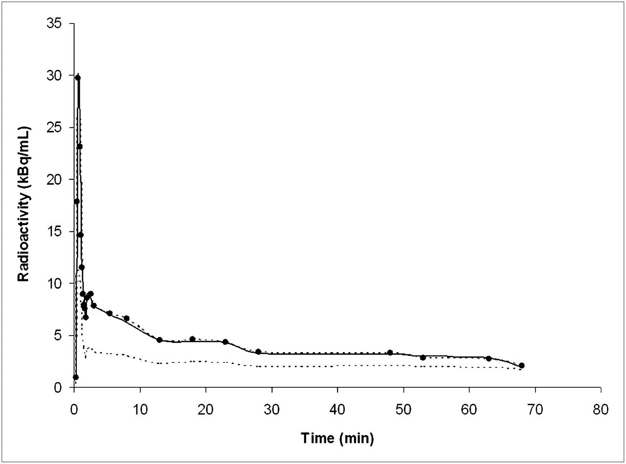
Comparison between reference time–activity curves (solid line) and automatic carotid time–activity curves (dashed line with dots), obtained using LMA in 8-mm-carotid phantom, corrected for spillover and partial-volume effect. Dashed line without dots is raw carotid time–activity curve not yet corrected for partial-volume effect.
The linear regression results for CMRglc for both phantoms are reported in Table 2. An excellent correlation was found between CMRglc obtained by manual and automatic carotid segmentation using LMA. Both manual and automatic image-derived CMRglc values correlated well with the original phantom values.
Correlation Between CMRglc Obtained by Arterial Sampling and Manual and Automatic Image-Derived Input Function After Correction for Partial-Volume Effect
Clinical Studies
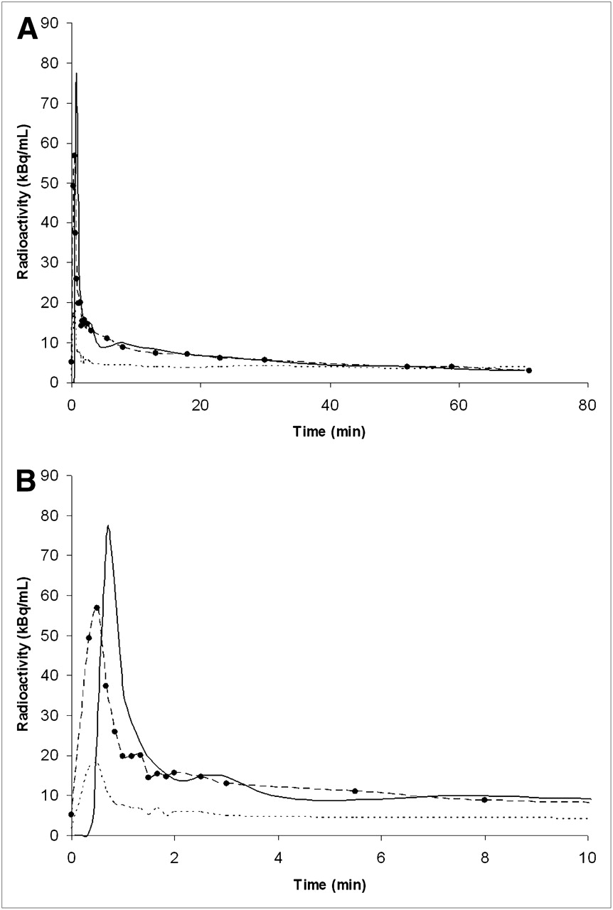
LMA was chosen for the clinical studies. The visual inspection shows that the internal carotids were successfully segmented in each patient. Figure 4 shows the results for 1 patient. Intracranial venous sinuses were segmented as well (data not shown). No significant differences were observed between time–activity curves, with and without correction for partial-volume effect, extracted from ROIs obtained by manual positioning and automatic segmentation using LMA (P < 0.001). Figure 5 compares arterial input function and automatic image-derived input function, obtained after partial-volume effect correction, for 1 subject. In all image-derived vascular time–activity curves from clinical data, both with manual and with automatic ROI placement, the peak height was underestimated, as compared with arterial plasma samples (mean value, −26%). However, the width of the peak was similar and no statistically significant difference was found in the total area under the curve between the image-derived and the reference input functions.
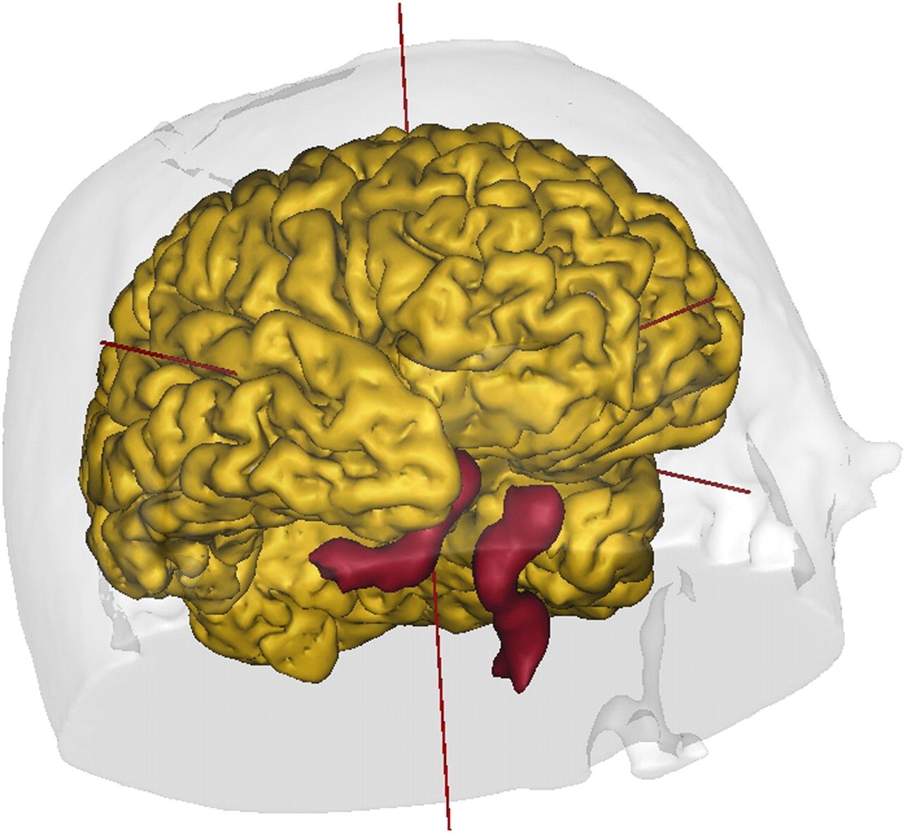
Internal carotid segmentation results using LMA in volunteer. Shown is right inferior view of MRI-derived 3-dimensional mesh of volunteer's brain. Segmented carotids are in red.

(A) Corrected image-derived input function obtained by automatic ROI placement in 1 subject (dashed line with dots), compared with arterial blood samples (solid line). Dashed line without dots represents uncorrected carotid time–activity curve. (B) Expanded view of first 10 min of same curve. Although late part of image-derived curve coincides well with reference values, peak is underestimated.
Of note, in all clinical studies the activity peak on the images occurred slightly earlier than the arterial peak (Fig. 5B), thus reflecting the different transit time to the carotids and to the radial arteries. However, this time difference has no consequences on the estimation of CMRglc (9).
The image-derived CMRglc values correlated well with those obtained by arterial sampling (Table 2).
Interobserver Variability
Visual analysis of the time–activity curves obtained from manually defined ROIs showed a good concordance between the 3 observers in most cases. ANOVA did not show statistically significant differences between the areas under the curve obtained manually by the 3 observers.
DISCUSSION
We have shown that the LMA algorithm effectively delineates internal carotids on dynamic PET images, faring better than 2 other existing segmentation algorithms, SCA and k-means. The time–activity curves thus obtained can be used, after correction for partial-volume effect and spillover, to calculate the input function for cerebral PET studies. Noteworthy is that LMA delineates intracranial venous sinuses as well, which have been validated for the estimation of image-derived input function by manual segmentation (10).
Segmentation of small vessels in PET images is challenging because of both their diameter, which may lie at the limit of the spatial resolution of modern PET cameras, and their tortuous shape. Therefore, small intracranial vessels have traditionally been segmented manually (8–10). In the present study, automatic segmentation using LMA yielded statistically similar results, in terms of ROI values and CMRglc quantification, to those obtained by manual segmentation.
The LMA segmentation algorithm has several advantages over the other 2 methods. First, LMA is a local method of segmentation, so that erroneous local estimations entail only local errors. In the case of k-means or SCA, each voxel that is affected by movement or reconstruction artifacts, even those at a distance in the matrix, contributes to the estimation of the organ kinetics. Second, our algorithm does not require that the number of classes in the images be selected before segmentation: the number of regions can be chosen in the final image at the end of the segmentation process. Third, LMA is 15–20 times faster than SCA and k-means (17). Indeed, no iterative process is required for estimation of the local mean kinetics, because they are extracted once in the core of each organ. Moreover, computational time for LMA is independent of the number of organs, whereas for SCA and k-means the time increases with the number of classes. With LMA, the automatic segmentation of internal carotids requires about 10–20 s per subject on a Dell computer running on a 1.86-GHz dual-core Xeon processor (Intel). Fourth, LMA implements a connectivity constraint; that is, spatially separated regions are considered different, even if the kinetics are similar. This allows one to correctly differentiate arterial and venous segments, provided that they are anatomically separated, as in the case of internal carotids and intracranial venous sinuses.
Besides the obvious advantage of requiring little effort from the operator, the use of automatic algorithms for ROI definition should in principle be preferred over manual delineation for 2 reasons. First, through selection of those voxels that are kinetically similar, only those regions that have a similar response can contribute to the averaging of the vascular time–activity curve. Thus, larger ROIs can be obtained, with better statistical properties and better signal-to-noise ratios (6,12). In the present study on phantoms, we obtained better results with LMA than with manual segmentation, as assessed by Q scores, although there was no significant difference in the estimation of CMRglc values. The most obvious explanation is that the algorithm can more accurately detect the boundary between the vascular structure and background tissues, as the algorithm is insensitive to variable levels of saturation in the image and to different color scales.
Second, automatic algorithms may obviate interobserver variability. However, in the present study, differences in areas under the curve obtained by the 3 observers were not statistically significant. One likely explanation is that carotids have a good signal-to-noise ratio in the early frames and are easily recognizable. Moreover, the small size of carotids would force the observers to define similar ROIs. Van der Weerdt et al. (6) obtained vascular time–activity curves by manually drawing ROIs on different cardiac and aortic structures. Their data show that the larger the vascular structure, the lower the interobserver reproducibility. Therefore, automatic algorithms should be the most useful for larger vascular structures.
To be used for CMRglc calculation in PET brain studies, internal carotid time–activity curves should be corrected for partial-volume effect. Predictably, as compared with reference values, estimation of CMRglc was on average more accurate in the phantom studies than in the clinical data. This greater accuracy is probably partly due to a more heterogeneous background tissue activity in clinical data, thus lowering the precision of corrections for spillover and partial-volume effect. Moreover, small movement artifacts are always possible during clinical studies.
On the image-derived curves of the healthy volunteers, we observed an underestimation of the early part of the curve, particularly of the peak height (Figs. 5A and 5B). Compared with the original study of Chen et al. (9), the estimations of the early curves in our study are somewhat less accurate, probably because of the coarser PET framing in our study. In fact, each PET frame corresponds to the integral of the signal over a time period. Conversely, for the phantom studies, each frame corresponds to a punctual detection at a given time. Therefore, the phantom peaks are fully resolved. A poor assessment of the early part of the curve precludes the possibility of a reliable estimation of the underlying rate constants of the kinetic model. However, the total area under the curve was not statistically different between image-derived input functions and reference arterial values. When using Patlak graphical analysis for estimation of the macroparameter K = K1k2/k2 + k3, errors in the estimation of the peak height entail only negligible variations on the final CMRglc values (9).
In contrast, a poor assessment of 18F-FDG activity at later times could be a major cause of CMRglc miscalculation. These errors are mainly due to partial-volume effects and spillover from surrounding tissues. Different image-based methods, aimed at correctly scaling the late part of the curve, have been proposed in the literature (8,10,22,23). However, the feasibility of CMRglc calculation without any blood sampling is currently being debated (24).
Therefore, for the present study, we chose a simple and straightforward method that relies on late venous blood samples to approximate the arterial radioactivity (9). Moreover, it must be remembered that venous blood sampling is the most accurate way to obtain the blood glucose concentration, which is required for CMRglc quantification.
CONCLUSION
The LMA segmentation algorithm allows accurate automatic delineation of internal carotids from dynamic PET brain studies with minimal manual, subjective effort. After correction for partial-volume effect, the main application would be the estimation of an image-derived input function.
Footnotes
-
COPYRIGHT © 2009 by the Society of Nuclear Medicine, Inc.
References
- Received for publication October 28, 2008.
- Accepted for publication November 24, 2008.


Jump to section
Related Articles
Cited By...
- No citing articles found.