


Abstract
Monte Carlo simulation can be particularly suitable for modeling the microscopic distribution of energy received by normal tissues or cancer cells and for evaluating the relative merits of different radiopharmaceuticals. We used a new code, CELLDOSE, to assess electron dose for isolated spheres with radii varying from 2,500 μm down to 0.05 μm, in which 131I is homogeneously distributed. Methods: All electron emissions of 131I were considered, including the whole β− 131I spectrum, 108 internal conversion electrons, and 21 Auger electrons. The Monte Carlo track-structure code used follows all electrons down to an energy threshold Ecutoff = 7.4 eV. Results: Calculated S values were in good agreement with published analytic methods, lying in between reported results for all experimental points. Our S values were also close to other published data using a Monte Carlo code. Contrary to the latter published results, our results show that dose distribution inside spheres is not homogeneous, with the dose at the outmost layer being approximately half that at the center. The fraction of electron energy retained within the spheres decreased with decreasing radius (r): 87.1% for r = 2,500 μm, 8.73% for r = 50 μm, and 1.18% for r = 5 μm. Thus, a radioiodine concentration that delivers a dose of 100 Gy to a micrometastasis of 2,500 μm radius would deliver 10 Gy in a cluster of 50 μm and only 1.4 Gy in an isolated cell. The specific contribution from Auger electrons varied from 0.25% for the largest sphere up to 76.8% for the smallest sphere. Conclusion: The dose to a tumor cell will depend on its position in a metastasis. For the treatment of very small metastases, 131I may not be the isotope of choice. When trying to kill isolated cells or a small cluster of cells with 131I, it is important to get the iodine as close as possible to the nucleus to get the enhancement factor from Auger electrons. The Monte Carlo code CELLDOSE can be used to assess the electron map deposit for any isotope.
To better understand the radiobiologic effects resulting from the use of an electron-emitting radiopharmaceutical, it is necessary to have an appropriate knowledge of the cellular distribution of the radiopharmaceutical and then to model the microscopic distribution of energy deposited in irradiated matter (1). Absorbed doses to targeted cancer cells play an important role in evaluating the relative merits of different radionuclides and pharmaceuticals.
Information on the biodistribution at the tissue, cellular and subcellular levels can be obtained by autoradiography (2), microautoradiography (3), or alternative techniques such as secondary ion mass spectrometry (4). Converting these data to absorbed dose distribution requires the use of analytic methods based on point-dose kernels or methods based on Monte Carlo radiation transport calculations (5–7).
For modeling the microscopic distribution of a local energy deposit, Monte Carlo code event-by-event simulations can be particularly suitable (7–10). The development of these track-structure codes necessitates accurate interaction cross sections for all electronic processes: ionization, excitation, and elastic scattering. The Monte Carlo track-structure code used here, named CELLDOSE, is based on cross sections published by Champion (8). All primary and secondary electrons are followed down to 7.4 eV.
In this article, we present the new Monte Carlo code, CELLDOSE, and use it to assess electron dose (and dose distribution) in spheres of various sizes containing 131I.
MATERIALS AND METHODS
We used the Monte Carlo code CELLDOSE to assess (a) the average electron dose “S values” for isolated water spheres, with radii varying from 2,500 μm down to 0.05 μm, in which 131I is homogeneously distributed; (b) the electron dose distribution inside the spheres; (c) the fraction of electron energy that is retained according to sphere size; and (d) the specific contributions of β−-particles and of monoenergetic electrons to the absorbed dose for each sphere.
CELLDOSE is a new computational code written in C. The main program consists of successive Monte Carlo random samplings among cumulative probabilities. These probabilities are precalculated and stored by way of raw and column data covering a large range of incident and ejected energies (10 eV–1 MeV) as well as ejection angles.
The energy and momentum transfers are then randomly selected and used by a large number of numeric subroutines, including integration and interpolation methods to describe the kinematics of the collisions induced by the primary particle as well as the secondary electrons created along the initial track.
In the present work the energy of each primary is randomly selected from the 131I decay spectrum, whereas its position is randomly chosen within the sphere simulated by assuming that 131I is homogeneously distributed. We took into consideration the whole spectrum of β-emission for 131I (by summing the 6 independent transition spectra, weighted according to their yields), as well as 108 internal conversion electrons, and 21 Auger electrons (Web site http://www-nds.iaea.org/nudat2; (11)). Figure 1 shows the primary electron spectrum of 131I decays.
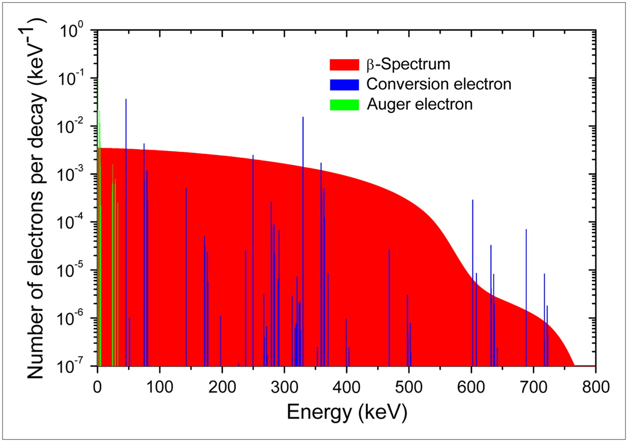
Mean primary electron spectrum of 131I decays.
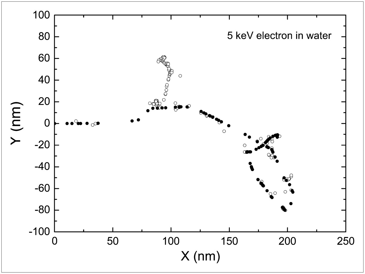
The full slowing-down histories for electrons are described and followed from their initial energy down to a few electron volts. Figure 2 shows an example of a 5-keV electron track.

Two-dimensional plot of a 5-keV electron track obtained with Monte Carlo code CELLDOSE. •, Inelastic interactions of primary electron. ○, Inelastic interactions of secondary electrons.
The coordinates and the energy deposits induced by all of the charged particles generated during the slowing-down of the incident electrons are stored by way of raw data to finally provide a complete 3-dimensional cartography.
Some assumptions underlying the present transport simulation and a brief description of Monte Carlo principles are given in the Appendix.
The program makes no use of additional library. It has been designed and performed on Linux x86 and x86-64 OEM (Original Equipment Manufacturer) workstations (Intel Pentium4-EM64T) compiled with Intel Compiler on Linux Debian.
Finally, the execution time strongly depends on the sphere size and on the statistics chosen. On average, the job running time was a few hours on a Pentium4-EM64T-3GHz with 1Go RAM memory.
A convivial version of CELLDOSE will be soon made available online.
RESULTS
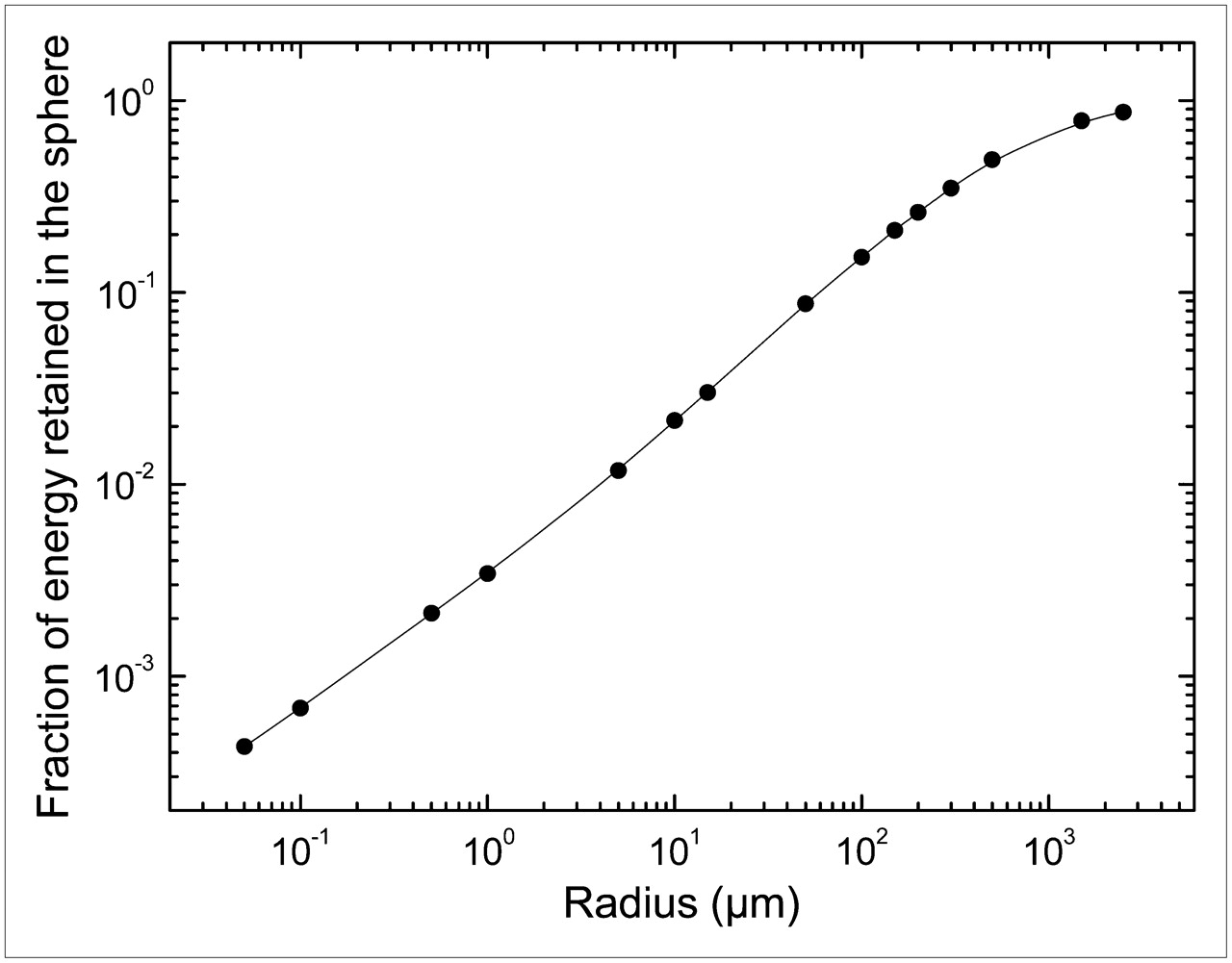
Table 1 gives the fraction of electron energy that is retained in each sphere. Figure 3 shows a plot of the fraction of energy retained versus the sphere radius.

Fraction of energy retained vs. sphere radius.
Fraction of Electron Energy Retained in Each Sphere and S Values: Comparison with S Values Reported by Goddu et al. and by Bardiès and Chatal
Table 1 also gives the S value (dose per disintegration) for each sphere. S values reported previously by Goddu et al. (12,13) and by Bardiès and Chatal (14), based on analytic methods, are quoted for comparison (Table 1). S values from Goddu et al. are slightly lower than ours (between −9.6% and +4.5%), whereas those from Bardiès and Chatal are slightly higher (+2.5% to +8.8%).
A comparison of our S values with those reported by Li et al., using a Monte-Carlo code, PARTRAC, is given in Table 2. Values reported by Li et al. (7) are slightly higher than ours (+1.5% to +10.3%).
Comparison of S Values in This Work with S Values of Li et al.
Figures 4A and 4B show dose distribution across a sphere of 500-μm radius. The dose was assessed in concentric spheric shells at equidistant intervals of 10 μm starting from the center. There is a continuous decrease in dose from the center to the external layer. The profile of dose distribution is normalized using as reference the dose at the center (Fig. 4A) or the average sphere dose (Fig. 4B).

Dose distribution across a sphere of 500 μm radius. Dose was assessed in concentric spheric shells at equidistant intervals of 10 μm starting from the center (first shell, 0–10 μm). Vertical dashed line indicates border of sphere. Profile of dose distribution is normalized using as reference dose at the center (A) or average sphere dose (B).
Some numeric values of dose distribution inside the spheres are also given in Table 3. The spheric shell in which the S value was similar to the average S value of the sphere is the one located at 400–410 μm from the center (Table 3). The dose at the center was 1.32 times higher than the average dose, whereas the dose at the outmost layer was 0.657 that of the average dose (Table 3; Fig. 4B). Thus, the dose in the outermost spheric shell was approximately half (49.8%) the dose at the center (Table 3; Fig. 4A).
Dose Distribution Inside a Sphere of 500 μm Radius Containing a Homogeneous Distribution of 131I
Table 4 gives for each sphere the relative contribution to the S values from β−-particles, Auger and internal conversion electrons. β− contribution ranged from 94.9% in the sphere with 2,500 μm radius to 22% in the 0.05 μm sphere. Auger electrons contribution was important only for small spheres. It varied from 0.25% for the largest sphere, to 76.8% for the smallest. The contribution from conversion electrons was 4.84% in the largest sphere, reached a maximum in the 50 μm radius sphere (9.1%), and stepped down to 1.2% in the smallest. Figure 5 shows plots of the relative contribution for each component according to the sphere radius.
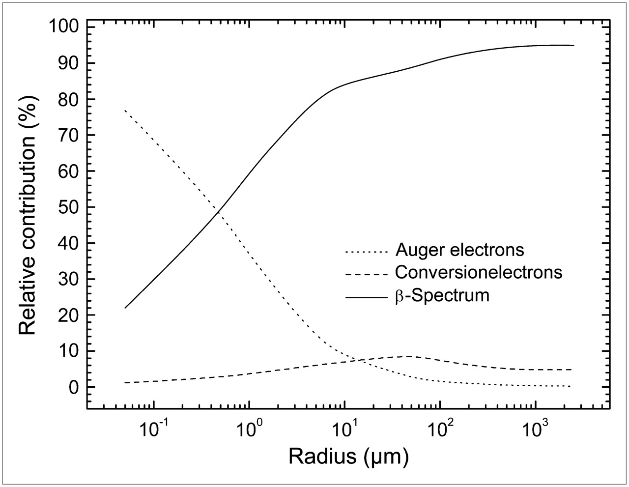
Plots of relative contribution from β−-particles, Auger electrons, and internal conversion electrons vs. sphere radius.
Relative Contribution to S Values from β−-Particles, Auger Electrons, and Internal Conversion Electrons
DISCUSSION
Traditional dose estimates have been based on average dose to whole organs (15,16). However, the MIRD Committee, as well as many authors, have brought into perspective the importance of dose distribution at the suborgan level (5,17,18) and at the cellular level (1,19,20). Monte Carlo code event-by-event simulations are particularly suitable tools to obtain a microscopic map of the energy deposited in irradiated matter. The great advantage of Monte Carlo track-structure simulation is that it is extremely flexible and can be adapted easily to new input data and to any geometry.
The Monte Carlo code CELLDOSE presented here can be used to assess the electron map deposit for most isotopes. The electron–water molecule interaction cross sections used (8) are valid for a wide energy range, 10 eV–1 MeV.
S values for isolated spheres of various sizes were obtained and compared with those reported previously. Our S values are in good agreement with analytic methods as published by Goddu et al. (12,13) and by Bardiès and Chatal (14), lying in between reported results for all experimental points (Table 1). Analytic methods use energy loss expressions for electrons derived from the experimental data of Cole on the relation between the energy and the continuous slowing-down range of monoenergetic electrons (21). S values from Goddu et al. are slightly lower than ours (except for their smallest sphere of 1-μm radius), whereas those from Bardiès and Chatal are slightly higher. The smallest radius investigated by Bardiès and Chatal was 10 μm. They stated that the point kernels used in their approach are valid beginning at 10 keV, which limits the validity for spheres with radii smaller than 10 μm (14).
We provide S values down to 0.05 μm radius. We did not calculate S values for smaller spheres for the following reasons:
The minimum electronic excitation potential of water molecules (7.4 eV) was chosen as the cutoff value. Below this threshold, the residual energy was assumed to be absorbed locally. Because the path of electrons of <10 eV is of the order of few angstroms, this approximation would introduce uncertainties smaller, or of the order of 1 nm, in the map of the energy deposits.
Electron–water molecule interaction cross sections were calculated in the gas phase approximation; the results are then extrapolated in the condensed phase by density scaling. For electrons of very low-energy (especially <20 eV), cross sections may differ between gaseous and condensed matter because of intermolecular bonds (22,23), although, at present, there are still no experimental data on liquid water. When examining energy deposit in very small volumes, and at a molecular (or DNA) level, the assumption that cells are simply composed of water is also an approximation, as the specific cross sections for cell components are not considered. Moreover, in such tiny volumes, the S value for 131I as an average dose per disintegration has little meaning, as the real dose would be variable, based on the kind of electron that is actually emitted.
Our S values are also in good agreement with those published by Li et al. (7), who simulated spheres with radii varying from 5 to 1,500 μm (Table 2). The authors used Monte Carlo techniques, and the S values reported by Li et al. were slightly higher than ours (1.5% to 10.3%). These differences could not be explained by the use of photons in addition to electrons in their work, as the fraction of photons that is absorbed is <1%, even for the largest sphere (24). Therefore, this small difference between our data and those of Li et al. remains unexplained.
Li et al. (7) characterized the dose distributions within spheres as constant values. However, contrary to these authors, we noted a continuous decrease in dose from the center to the external layer. Figure 4 shows the microscopic distribution of dose across a sphere of 500 μm radius. The S value for the outmost layer was 49.8% of the S value in the center (Table 3; Fig. 4A) and 65.7% of the average S value (Table 3; Fig. 4B). The center is surrounded by the radioactive medium covering a space angle of 4 π, whereas the rim receives radiation from slightly less than half that space angle. A dose gradient was also reported by Hartman et al. (19). That Li et al. did not record a dose gradient from the center to the periphery and the inconsistent pattern of dose distribution (clearly apparent in the 500 μm radius sphere in their figure 6) probably results from low statistics. For example, for the 500 μm sphere, these authors used 50,000 decays, whereas we used 17,000,000 decays to obtain a fine map of the dose distribution.
A dose gradient should have implications in targeted radionuclide therapy. The dose to a tumor cell will depend on its position in the metastasis. In the case of the homogeneous distribution of radioactivity in the 1-mm metastasis shown in Figure 4B, cells located at the border of the tumor will receive only 66% of the average tumor dose (those cells located at the center would receive 132%).
Another specificity of targeted radiotherapy compared with external beam radiotherapy is the relation between the fraction of retained energy and tumor size. The absorbed fraction of electrons from 131I reaches 95% for a sphere of 1 g with a 6.2 mm radius (25). However, this fraction will decrease with decreasing sphere size, as shown in Table 1 and Figure 3, indicating that 131I may be less efficient for treatment of small tumor targets (micrometastases, tumor cell clusters, and isolated tumor cells), as has also been reported by Hindorf et al. for lymphoma cells (26). Indeed, a substantial proportion of the disintegration energy escapes and is deposited outside the tumor volume. Table 1 shows that the retained fraction of emitted electron energy was 87.1% for a sphere of 2,500 μm radius, 49.2% for a sphere of 500 μm radius, 8.73% for a sphere with 50 μm radius (cell cluster), and only 1.18% in a sphere with 5 μm radius (cell size).
Thus, for small metastases, knowledge of the percentage uptake per gram is not sufficient and the dose calculation has to be corrected by the fraction of the electron energy that is actually absorbed. Therefore, for a given 131I concentration that delivers a dose of 100 Gy to a micrometastasis of 2,500 μm radius, the same concentration would deliver roughly 10 Gy in a cluster of 50 μm, and only 1.4 Gy in an isolated cell, assuming that the distribution is homogeneous. However, this consideration that applies to a homogeneous distribution may need to be adapted in the case of a heterogeneous distribution when cross fire becomes necessary to overcome tissue heterogeneity.
Previous studies have shown that when trying to kill isolated cells or a small cluster of cells with 131I it becomes important to get the iodine as close as possible to the nucleus and to DNA (19,20). Using cell labeling with 131I-iododeoxyuridine, Neti and Howell (20) reached the conclusion that the self-dose to the nucleus that comes from 131I-IdU has a relative biological effectiveness (RBE) of about 3.3 compared with cross dose to the nucleus from 131I in surrounding cells. The self-dose corresponding to 37% survival (D37) for V79 cells (the cell nucleus had a radius of 4 μm) was 1.2 Gy, whereas the corresponding 37% survival for the cross dose was 4 Gy.
A higher toxicity for DNA-incorporated 131I than for the cross dose arising from 131I decays in surrounding cells suggests a high contribution from low-energy electrons with a highly localized energy deposit. Our results may explain why the self-dose for 131I-IdU is more toxic per unit dose than the cross dose. From Table 4, it can be seen that for a sphere radius of 5 μm, the Auger contribution to the dose is 13.4% and, for a 1-μm radius this contribution reaches 36.5%. As this part of energy is deposited close to its site of origin, the real dose received by DNA can be much higher than the average dose to the nucleus.
CONCLUSION
S values for 131I in spheres of various sizes were in agreement with previously published values. From this simple model it was inferred that the dose to a tumor cell will depend on its position in a metastasis. Cells located at the border of the tumor will receive only half the dose at the center. It is also shown that for the treatment of very small metastases, 131I may not be the isotope of choice. A substantial fraction of electron energy will escape these tumors, reducing the tumor dose and contributing to nonspecific toxicity. We also presented data pointing to the specific contribution of Auger electrons in small spheres. When trying to kill isolated cells or small cluster of cells with 131I, it is important to get the iodine as close as possible to the nucleus to get the enhancement factor from Auger electrons.
The Monte Carlo code CELLDOSE presented here can be used to assess the electron dose map deposit for any isotope. In future work we will show how results can be extended from isolated spheres to a complex multisource geometry.
APPENDIX
Some Assumptions Underlying the Present Transport Simulation (8)
-
Energy loss results essentially from inelastic collisions (ionization and excitation) because the energy loss induced by elastic scattering is very small—that is, of the order of millielectron volts
-
Auger electron after an inner-shell ionization is assumed to be isotropically emitted.
-
Bremsstrahlung production is negligible in the energy range considered.
-
Relativistic corrections were introduced in the present work.
-
Water molecules are assumed to be uniformly distributed and treated in the gas-phase approximation. Then, the results are extrapolated in the condensed phase by a simple density scaling. Minor differences resulting from differences in ionization potentials between the gaseous and liquid state of water are neglected.
-
Density correction can be introduced to fit that of the studied tissue. Here we used ρ = 1 g·cm−3.
-
The minimum electronic excitation potential of water molecules (7.4 eV) was chosen as the cutoff value. Below the cutoff energy of 7.4 eV, the residual energy was assumed to be absorbed locally.
Monte-Carlo (MC) Principles (8)
The transport simulation in essence comprises a series of MC sampling steps that determine:
the distance to the next interaction,
the type of interaction that occurred at the point selected,
the energy and direction of the resultant particles according to the type of interaction selected.
Thus, after defining the primary particle's initial parameters, such as particle type and its energy, the code determines the free path traveled by direct random sampling (MC sampling) according to the sum of all of the total interaction cross sections relative to all of the electronic processes included in the simulation. The particle is then transported to its new position. By applying again direct MC sampling according to the relative magnitude of the individual total interaction cross sections (elastic scattering, ionization, and excitation cross sections), the type of collision is randomly determined:
If the interaction is elastic, then by applying the random MC sampling according to the singly differential cross sections, the scattered direction is determined at the appropriate electron incident energy Einc, which remains quasi-unchanged because the energy transfer induced during the elastic scattering is very small (in the order of millielectron volts).
In the case of ionization, then first, by applying the random MC sampling according to the singly differential cross sections, the kinetic energy of the ejected electron Ee is determined. Following the choice of Ee, application of direct MC sampling according to the relative magnitude of the partial total ionization cross sections (at Ee) the ionization potential IPj is determined. The particle energy is reduced by Ee + IPj, whereas the ejected and scattered directions are determined according to the 5-fold and triply differential cross sections, respectively (5DCS and TDCS, respectively). Indeed, all geometric parameters (the polar and azimutal angles of the ejected and scattered electrons, θe, ϕe, θs, and ϕs, respectively) are randomly sampled from successive integrations of the 5DCS (denoted σ(5)) defined by: σ(5) = d5σ/dΩsdΩedEe, where Ωs corresponds to the scattered direction (dΩs = sinθsdθsdϕs), Ωe the ejected direction (dΩe = sinθedθedϕe), and Ee the energy transfer. Then, the particular ionization potential IPj is stored as locally deposited energy.
If, finally, excitation is decided, direct MC sampling is applied according to the relative magnitude of all partial excitation cross sections for determining the transition level n. The particle energy is reduced by En, whereas the incident direction remains “unaltered” (27). Similar to the case of ionization, the particular excitation potential En is stored as locally deposited energy.
All of these steps are consecutively followed for all resultant particles until their kinetic energy falls below the predetermined cutoff value (Eth = 7.4 eV). Subthreshold electrons are assumed to deposit their energy where they are created. This approximation introduces uncertainties smaller, or of the order of 1 nm, in the map of the energy deposits. In these conditions, the code is able to provide by way of row data the coordinates of all interaction events as well as the type of collision together with the energy loss, the energy deposited at each interaction point, and the kinetic energy of the resultant particle(s) in the case of inelastic collision.
As an example, Figure 2 shows a 2-dimensional plot of a 5-keV electron track.
Footnotes
-
Elif Hindié, MD, PhD, Service de Médecine Nucléaire, Hôpital Saint-Louis, 75475 Paris Cedex 10, France. E-mail: elif.hindie{at}sls.aphp.fr
-
COPYRIGHT © 2008 by the Society of Nuclear Medicine, Inc.
References
- Received for publication July 12, 2007.
- Accepted for publication October 12, 2007.


Jump to section
Related Articles
Cited By...
- Membrane and Nuclear Absorbed Doses from 177Lu and 161Tb in Tumor Clusters: Effect of Cellular Heterogeneity and Potential Benefit of Dual Targeting--A Monte Carlo Study
- Membrane and Nuclear Absorbed Doses from 177Lu and 161Tb in Tumor Clusters: Effect of Cellular Heterogeneity and Potential Benefit of Dual Targeting--A Monte Carlo Study
- Multimodal Imaging of 2-Cycle PRRT with 177Lu-DOTA-JR11 and 177Lu-DOTATOC in an Orthotopic Neuroendocrine Xenograft Tumor Mouse Model
- Dose Deposits from 90Y, 177Lu, 111In, and 161Tb in Micrometastases of Various Sizes: Implications for Radiopharmaceutical Therapy
- Cellular Dosimetry of 111In Using Monte Carlo N-Particle Computer Code: Comparison with Analytic Methods and Correlation with In Vitro Cytotoxicity
- Reply: 131I Radiation Dose Distribution in Metastases of Thyroid Carcinoma
- 131I Radiation Dose Distribution in Metastases of Thyroid Carcinoma