


Abstract
Many quantitative imaging protocols that make use of a metabolite-corrected arterial input function require the use of a mathematic model to describe the rate of metabolism of the radioligand. Commonly, parametric models are fit to metabolism data and then the fitted model is used to correct the plasma input function. 11C-WAY 100635 is a rapidly metabolized radioligand used extensively in mapping the 5-hydroxytryptamine receptor 1A system. Methods: To evaluate the adequacy of fit of 4 metabolite models, we examined data from 92 subjects who received an injection of 11C-WAY 100635, were imaged with PET, and underwent measurement of total plasma concentration and metabolites. The performance of these models was assessed according to residual plots, as well as fit and information criteria. Results: The study showed that the choice of model has a substantial effect on the resulting estimates of outcome measures. Conclusion: Among the models considered, the Hill model provides the best fit across all criteria.
The radioligand 11C-WAY-100635 is used extensively in imaging the 5-hydroxytryptamine receptor 1A system (1–5). In such studies, the method for estimation of binding potential (maximum number of binding sites divided by dissociation constant) that involves the fewest assumptions requires determination of the metabolite-corrected arterial input function. Typically, total radioactivity counts in the plasma are corrected for the rate of metabolism of the injected “parent” (unmetabolized radiotracer). In the case of the PET ligand 11C-WAY-100635, metabolism is rapid, with nearly 80% of the parent compound being metabolized within 5–15 min.
For accurate quantification of the binding potential, we have shown that a minimum of 110 min of emission scanning are required (6). Metabolites cannot be determined reliably at late times because of low levels of parent compound; low counting rates decrease confidence in count estimates; and 11C decays relatively quickly: For these reasons, the metabolite curve is typically fit by a parametric model and extrapolated to late times according to the fitted model.
Models that have been used for this purpose include 1-exponential (6), 2-exponential with 1 time constant constrained (7), 3-exponential (8,9), multiexponential (10,11), and a Hill function (12,13).
We examined 4 candidate models for the rate of metabolism of the parent compound in plasma over time. Model fit was assessed using residual sum of squares, Akaike information criterion (AIC) (14), and residual plots.
MATERIALS AND METHODS
Data Description
We considered data from 92 subjects recruited in an ongoing neuroreceptor imaging study. Imaging and measurement of metabolites were performed as described previously (6). Briefly, after acetonitrile extraction of the plasma, samples were separated into parent and 1 polar metabolite peak by high-pressure liquid chromatography on 5 samples. Extraction was measured at every time point and did not vary with time. The rate of metabolism is presented as a ratio of the area under the curve of the unmetabolized compound peak divided by the total unmetabolized and metabolized peak. In other words, the fraction of unmetabolized compound is where vi is the radioactivity count, corrected for background and decay, under peak i. The metabolites are eluted from the column first and collected in tubes (fractions) numbered 1 through 3. The parent is eluted later, with no overlap between the parent and metabolite, and collected in fractions 4 and 5. The fractions are then counted in the well counter, and the percentage of unmetabolized compound is calculated as above.
Modeling Metabolite Data
We considered 2 types of models. One approach is to model the proportion of unmetabolized parent ligand. An alternative is to model the concentration of the parent compound directly with a physiologic model of metabolism. At time t, we used Cp(t) and Cmet(t) to denote the concentrations of parent compound and metabolite, respectively. Total concentration is given by  . Thus, “proportion models” are fit to describe the fraction
  ; the kinetic modeling alternative is to fit the
  measurements directly.
Proportion Models.
Observed fractions  taken at corresponding time points are modeled as
  , where
  represents the noise. Proportion models are constrained in 3 ways. Specifically, because the compound is injected at time zero, it is assumed that the compound is not metabolized and hence
  (the first constraint). After that, the compound is continuously metabolized (the second constraint), and its metabolism is irreversible (the third constraint).
The first proportion model considered is the 1-exponential model: Eq. 1The restrictions are satisfied provided that
  and
and  .
.
Another common model is the 2-exponential model: Eq. 2We arbitrarily let
  represent the larger of the 2 time constants (i.e.,
  ). Restrictions on this model are satisfied if
  .
.
The third model for metabolite fraction considered is the Hill model (15): Eq. 3for which we require
  ,
,  , and
, and  .
.
A Kinetic Model.
Knowledge of the kinetics of the metabolism process may improve our ability to model the data. To our knowledge, no published paper using WAY100635 has applied a kinetic model to fit the metabolite function, but it seems important to consider at least 1 kinetic model for comparison's sake. We considered a basic 2-compartment kinetic model that allows for 1 metabolite as diagrammed in Figure 1. Though alternative kinetic models could be fit, model complexity is limited by the small number of data points per subject.

Diagram of kinetic model. Parent compound begins in plasma and passes to tissue compartment (thought to be composed primarily of liver but could also include kidneys and other tissues). Some compound is metabolized and moves to “met” compartment; rest is excreted back to blood without being metabolized. Rate parameters k1– k4 are assumed to be nonnegative.
The total concentration of radioactivity in the plasma is measured over time through plasma analysis. The concentration of metabolite  is measured through metabolite analysis, but
  cannot be observed directly. In our study, the metabolite data consist of the fraction of unmetabolized compound at
  specific time points (
 ), and the plasma data consists of
  time points and corresponding total concentrations of radioactive substances (i.e.,
  ).
).
The system of differential equations corresponding to Figure 1 in terms of rate parameters is
 The solution for
  is given by
 Eq. 4where ⊗ denotes convolution.
The total concentration  in Equation 4 was estimated from a plasma data model. Our plasma model comprised 2 pieces: After the injection, the concentration of the compound in plasma increased linearly for a short time to its peak value; after peaking, the concentration fell off according to a sum-of-exponentials model (6). The linear rise in the plasma function until the peak was a fairly crude representation of the true plasma concentration curve, but because this interval was small relative to total scanning time (about 1%), it makes little difference in the resulting model estimates. Once the total plasma data are fit to this model, the estimated plasma concentration function is plugged in for estimating
  .
.
Weighting.
The data used for the fitting are computed as ratios of radioactive counts in each fraction. In general, the fraction of unmetabolized (parent) compound is computed for a given time as where I represents an index set. For our data, indices range from 1 to 5 and I = {4, 5}.
The γ-counter (1480 Wizard 3M Automatic γ-Counter; Wallac) provides both the  values and an estimate of their SD. Using these quantities, estimates of the SD of the fractions can be computed using the so-called delta method. If each
  denotes the SD of the corresponding
  measurement and the
  's are taken to be independent, then the variance of Y is approximated according to
 Eq. 5This is used to determine the weights used in model fitting.
Model-Fitting Algorithm.
Standard iterative nonlinear regression methods are used for the model fitting: Eq. 6where β is the vector of the parameters in the models and
  is computed as
  according to Equation 5.
RESULTS
Visual Analysis of Model Fits
Figure 2 gives example fits for each model for a specific dataset. For the kinetic model, to equalize the model-fitting procedure (to allow a more direct comparison), we computed the corresponding fraction  by
by where
where  comes from Equation 4 and then is fit using Equation 6. Though the fitting is done using the fractional data, results are displayed using metabolite concentration data. The 2-exponential model clearly undershoots the later time points, because the 2-exponential model does not contain a constant term and is thus constrained to go to zero rapidly, even when the data do not justify this (as in this example). The data were also fit with a 2-exponential model with constant (results not shown), but the fitting procedure was rather unstable (many parameters with few data points) and for almost all subjects, one of the exponential terms had a zero coefficient, providing no improvement over the 1-exponential model.

Fitted data for all models for 1 subject's data. Plots show fitted unmetabolized fraction vs. observed data.
Comparisons Based on Fit Diagnostics
We also compared weighted residual sum of squares and AIC for each model across all datasets. AIC (14) attempts a compromise between model fit and parsimony by imposing a penalty for additional model parameters. For normally distributed errors, the criterion is AIC = nlog(weighted residual sum of squares/n) + 2M, where n is the number of data points and M is the number of model parameters.
Figure 3 shows box plots for AIC values corresponding to each candidate model; corresponding box plots for log(weighted residual sum of squares) are similar and not shown. On the basis of these measures, the Hill model fits the data best among the models considered.
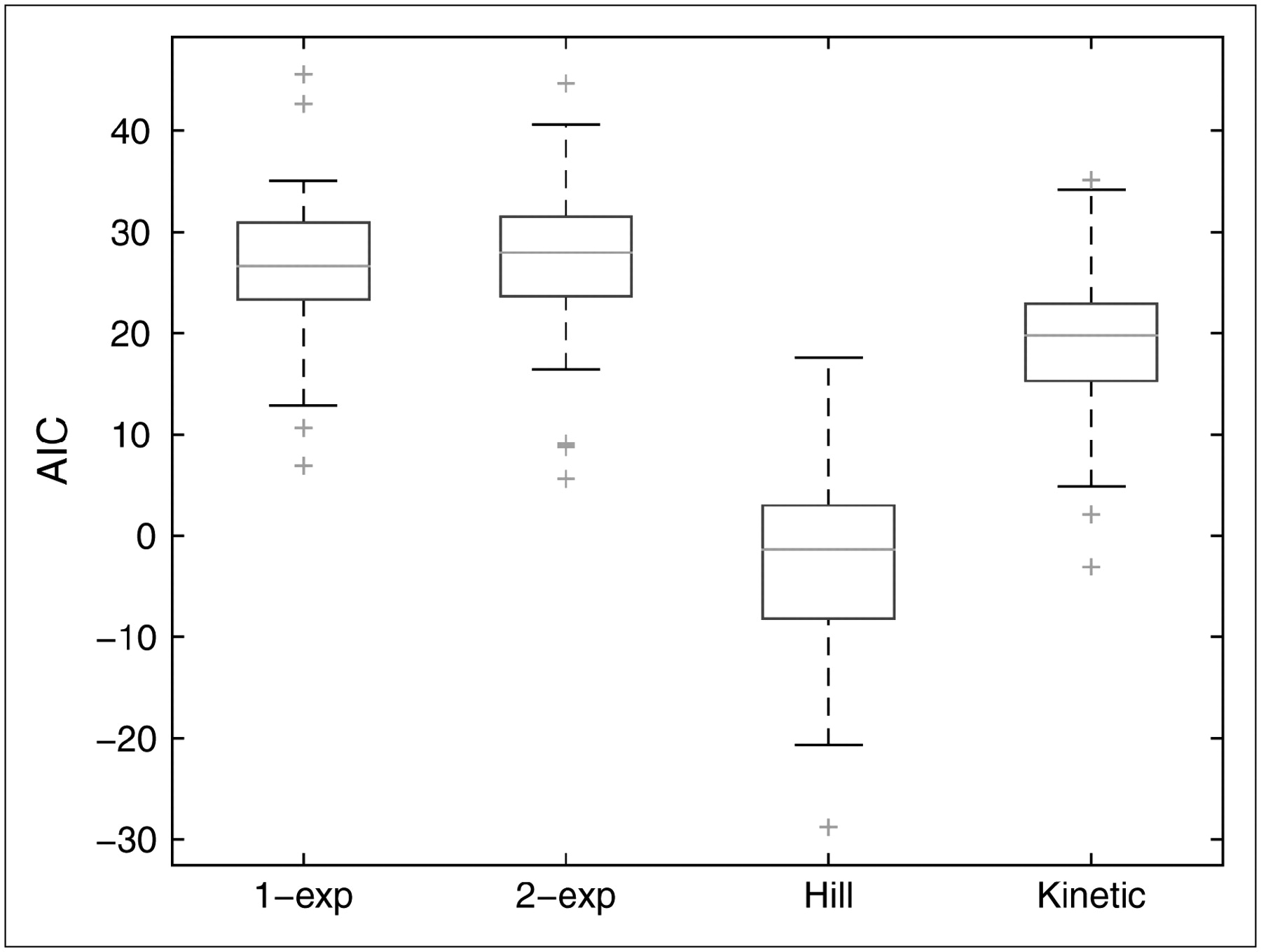
Box plots of AIC values for 1-exponential, 2-exponential, Hill, and kinetic models. One- and 2-exponential models have similar results, and kinetic model has smaller values than exponential models. Compared with the others, Hill model tends to have much smaller values: Maximum AIC value is less than median for kinetic model and less than 25th percentile for other models. exp = exponential.
Residual Analysis
If the model fits well, at least in large datasets, residuals for each dataset should have an approximate normal distribution with a mean of zero. We had no more than 6 observations in each dataset and thus could not expect residuals to have a distribution close to normality. However, for an appropriate choice of model, we would expect residuals to be centered on zero and to be nearly symmetric.
In a typical regression analysis, many observations are pooled to fit a model and all residuals are plotted together in a single plot. In our present study, data from each subject were fitted separately. In such a situation, we search for patterns among independent residuals by pooling across all subjects separately for each time point.
All residuals from all 92 subjects are displayed simultaneously in Figure 4. On the basis of both absolute size of residuals and distribution of residuals about zero, the Hill model would be preferred.

Graph of weighted residual for each model. For better visual display, points are spread out by adding small amount of gaussian noise in x direction. For 1- and 2-exponential models, residuals tend to fall only on one side of zero at each time point. Means of residuals are relatively far from zero, and distributions of residuals are, in general, rather asymmetric and heavily skewed. For kinetic model, similar problems exist. Residuals for Hill model look more reasonable: They are evenly scattered around zero, and their distributions are fairly symmetric. Although, at first 2 time points, residuals are skewed to one side of zero, they are all quite small relative to those of other models.
Effect on Kinetic Outcome Measures
A crucial question about metabolite modeling is whether the choice of model makes a difference for subsequent region-of-interest or voxel-level analysis. Therefore, we compared the resulting biologic parameters binding potential (BP1) and volume of distribution (VT) that resulted from different metabolite models.
For each candidate model, the resulting estimated metabolite-corrected plasma concentration curve was used as the input function for subsequent kinetic modeling of PET data. This procedure was applied to all 87 complete datasets to estimate total equilibrium VT (using a 1-tissue kinetic model) for cerebellum, and BP1 (using a 2-tissue constrained model) (6) for 4 regions: amygdala, hippocampus, cingulate, and parietal lobe.
The effect of the metabolite modeling is summarized in Table 1. To test for significance of the differences, paired t tests and Wilcoxon signed-rank tests were applied. Results are given in Table 2. All P values are small, indicating that the choice of metabolite model had a highly significant impact on resulting outcome measures derived from the imaging data.
BP1 Measurements Using Each of the 4 Candidate Models on 4 Brain Regions, Along with VT Estimates for Cerebellum
Paired t Tests and Signed-Rank Tests for Testing Difference Between BP1 and VT Estimates from Different Models
DISCUSSION
Having an arterial input function for modeling of dynamic PET data can be a great help, provided that the input function is measured and modeled appropriately. Key to the validity of the input function is correctly accounting for the metabolism process of the ligand. Thus, it is of vital importance to ensure that the model used to describe metabolism is adequate.
We considered only 1 kinetic model, though others are possible. Huang et al. (16) presented the kinetic model building procedure and model formulas for the general case, including the case of multiple metabolites. Andree et al. (17) showed that WAY100635 has more than 1 metabolite in humans. However, they also pointed out that only 1 metabolite (11C-desmethyl-WAY-100635) can be used as a radioligand for central 5-hydroxytryptamine receptor 1A; other metabolites are more polar and not likely to pass the blood–brain barrier. Osman et al. (18) observed another significant polar metabolite in some experiments—11C-cyclohexanecarboxylic acid—along with some other metabolites that were more polar still. Thus, with the exception of 11C-desmethyl-WAY-100635, no metabolites are expected to bind strongly to 5-hydroxytryptamine receptor 1A. Even if the radioactive acid metabolite binds nonspecifically, it is in low levels and cleared rapidly (in about 5 min). On the basis of these considerations, as well as the obvious limitation on the complexity of models that can be fit with 6 data points, we concluded that the kinetic model considered in the data would be an appropriate candidate for these data.
CONCLUSION
Among those considered, the Hill function was the model of choice to describe the metabolism of 11C-WAY-100635, and the impact of model choice was confirmed by the analysis on BP1 and VT data, demonstrating the need to carefully select an appropriate metabolite model in analyzing PET data.
Acknowledgments
This work was supported in part by MH62185 and NARSAD.
Footnotes
-
COPYRIGHT © 2007 by the Society of Nuclear Medicine, Inc.
References
- Received for publication November 14, 2006.
- Accepted for publication March 16, 2007.


Jump to section
Related Articles
Cited By...
- Modeling Strategies for Quantification of In Vivo 18F-AV-1451 Binding in Patients with Tau Pathology
- Quantification of 11C-Laniquidar Kinetics in the Brain
- In Hot Blood: Quantifying the Arterial Input Function
- Modeling Considerations for 11C-CUMI-101, an Agonist Radiotracer for Imaging Serotonin 1A Receptor In Vivo with PET