


Abstract
The toxicity of red bone marrow is widely considered to be a key factor in restricting the activity administered in molecular radiotherapy to suboptimal levels. The assessment of marrow toxicity requires an assessment of the dose absorbed by red bone marrow which, in many cases, requires knowledge of the total red bone marrow mass in a given patient. Previous studies demonstrated, however, that a close surrogate—spongiosa volume (combined tissues of trabecular bone and marrow)—can be used to accurately scale reference patient red marrow dose estimates and that these dose estimates are predictive of marrow toxicity. Consequently, a predictive model of the total skeletal spongiosa volume (TSSV) would be a clinically useful tool for improving patient specificity in skeletal dosimetry. Methods: In this study, 10 male and 10 female cadavers were subjected to whole-body CT scans. Manual image segmentation was used to estimate the TSSV in all 13 active marrow–containing skeletal sites within the adult skeleton. The age, total body height, and 14 CT-based skeletal measurements were obtained for each cadaver. Multiple regression was used with the dependent variables to develop a model to predict the TSSV. Results: Os coxae height and width were the 2 skeletal measurements that proved to be the most important parameters for prediction of the TSSV. The multiple R2 value for the statistical model with these 2 parameters was 0.87. The analysis revealed that these 2 parameters predicted the estimated the TSSV to within approximately ±10% for 15 of the 20 cadavers and to within approximately ±20% for all 20 cadavers in this study. Conclusion: Although the utility of spongiosa volume in estimating patient-specific active marrow mass has been shown, estimation of the TSSV in active marrow–containing skeletal sites via patient-specific image segmentation is not a simple endeavor. However, the alternate approach demonstrated in this study is fairly simple to implement in a clinical setting, as the 2 input measurements (os coxae height and width) can be made with either pelvic CT scanning or skeletal radiography.
The objective of molecular radiotherapy treatment planning is to determine the appropriate activity level of the therapy agent to be administered to an individual patient so as to ensure an effective response in the targeted diseased tissue while minimizing toxicities to nontargeted normal organs and tissues. The dose-limiting toxicity most frequently encountered in molecular radiotherapy, in particular, radioimmunotherapy, is myelosuppression for protocols that do not provide a priori for hematopoietic stem cell support (1). Dose–response relationships determined from data in human clinical trials therefore are sought for use in anticipating marrow toxicity in future patients, with the assumptions that consistent dosimetric analyses are conducted (2,3) and that other biologic modifying factors are considered (4). Recent and comprehensive reviews of the marrow dosimetry techniques currently used in clinical medicine may be found in articles by Stabin et al. (5), Sgouros (6), and Siegel (7).
Once marrow activity levels are assessed in a patient, through either blood-based (8) or image-based (9) methods, estimates of doses absorbed by red (hematopoietically active) bone marrow may be made by use of radionuclide S values for skeletal tissues assigned to a reference patient or anatomic phantom (10–12). When the radiolabeled agent does not bind to marrow cellular components, reference phantom S values may be used for skeletal dosimetry without an explicit need to assign or estimate the total red bone marrow (RBM) mass in the individual patient, as shown by Shen et al. (13). As discussed by Siegel (7), however, a total RBM mass estimate is required when marrow or bone tissue is targeted by the therapy agent. The conventional approach used in nuclear medicine is to make this estimate under the presumption that the total RBM mass within the skeleton is scaled linearly with the total body mass, as follows: Eq. 1In Equation 1, mRBM is the mass of the total RBM in either the patient or the reference phantom and TBM is the total body mass of the same individual or phantom. Stabin et al. (5) noted, however, that lean body mass might be a more appropriate scale for RBM mass estimates because lean body mass excludes the mass associated with storage fat, as follows:
 Eq. 2
Eq. 2
In 2002, studies by Bolch et al. (14) and by Shen et al. (15) independently suggested the use of trabecular spongiosa volumes (combined tissues of bone marrow and bone trabeculae in cancellous bone) as clinically useful scales for reference S values in skeletal dosimetry. Using 3-dimensional (3D) image-based radiation transport in the femoral and humeral heads, Bolch et al. (14) demonstrated close agreement between patient-specific and spongiosa volume–scaled energy-dependent radionuclide S values for electron energies above ∼100 keV. Shen et al. (15) further showed significantly improved correlations between RBM absorbed dose and observed myelotoxicity when the dose estimates were adjusted by patient-specific measurements of spongiosa volumes within the lumbar vertebrae. Both of these studies made the implicit assumption that ratios of RBM masses in skeletal region x are closely approximated by corresponding ratios of their trabecular spongiosa volumes, as follows: Eq. 3In Equation 3, SV is the spongiosa volume, MVF is the marrow volume fraction of the spongiosa, CF is the marrow cellularity factor (fraction of marrow volume that is hematopoietically active), and ρ is the tissue density. Equation 3 demonstrates that the ratio of spongiosa volumes is equivalent to the ratio of red marrow masses under the condition that the marrow volume fraction and the marrow cellularity of the patient are faithfully represented in the reference patient. The studies of Bolch et al. (16) and Watchman et al. (17) demonstrated that reference skeletal models can now be made to explicitly account for marrow cellularity in reference patient radionuclide S values, although this is not yet current clinical practice. Furthermore, MRI techniques are available to noninvasively assess marrow cellularity in individual patients (18–20). Consequently, cancellation of the cellularity factor terms in Equation 3 can be justified by proper selection of the reference S values matched to the patient's marrow cellularity assessed throughout the skeleton. Cancellation of the marrow volume fraction terms must still be justified, but the marrow volume fraction term has been shown to be important only for very low-energy–emitting radionuclides (mean β-energies of <100 keV) (14).
The purpose of the present study was to develop a clinically feasible regression model for predicting in a given patient the cumulative volume of trabecular spongiosa found across all major skeletal sites known to contain RBM in an adult (21). Accordingly, we defined the total skeletal spongiosa volume (TSSV) in the present study as encompassing the axial skeleton (trunk and head) and the proximal femora and humeri of the appendicular skeleton (as the distal extremities contain primarily inactive, or yellow, bone marrow in the adult). TSSV data for the regression analysis were taken from detailed image segmentation of whole-body CT scans of 20 cadavers (10 males and 10 females). Dependent fitting parameters included the total body height and 14 skeletal size measurements, with particular attention to sites used clinically for direct imaging of marrow activity uptake in molecular radiotherapy (9).
MATERIALS AND METHODS
Cadaver and Image Acquisition
With the cooperation of the State of Florida Anatomic Board at the University of Florida, 20 cadavers were selected for whole-body CT. Selection criteria included a trauma-related cause of death or a death that did not result in prolonged or progressive disease. In both cases, the skeletal structure of the individual was believed not to be altered from its normal age-dependent state. The body donation records used in cadaver selection do not contain the total body masses either before or after death. Additionally, the embalming process often prevents an accurate total body mass estimate after receipt of an individual by the Anatomic Board. Accordingly, premortem total body masses were estimated through visual inspection by the senior laboratory technician. These data, however, were for internal reference only and were not used in the regression analysis.
With the cooperation of the Department of Radiology at the University of Florida, each cadaver was subjected to a series of whole-body CT scans acquired with a Siemens Sensation 16 CT scanner. The slice thickness for the first 10 cadavers was 1 mm, and the in-plane pixel resolution was 977 μm. The number of slices to be analyzed in the 1-mm datasets was on the order of 1,000. In an effort to reduce analysis time to a more manageable magnitude, the slice thickness was increased to 2 mm for the remaining 10 cadavers in the study. The in-plane pixel resolution for the 2-mm datasets ranged from 936 to 977 μm.
Spongiosa Volume Estimation
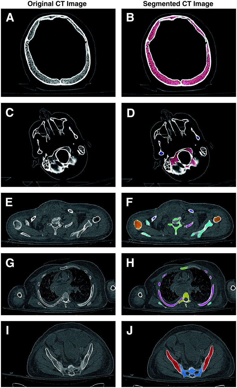
Image segmentation of the CT datasets was manually performed with a user-written Interactive Data Language (IDL version 6.0; ITT Visual Information Solutions, Inc.) software program (22). This program allows the user to create a computer file consisting of contours of each slice superimposed on CT image slices. Within each slice of the contour file, an interactive pen display was used to outline selected skeletal regions for each CT slice. The interior of the outlined skeletal region was assigned a segmentation or tag value within the contour file; each tag value corresponded to a unique color and skeletal site (for example, cranium, ribs, and cervical vertebrae), as shown in Figure 1. The numbers of voxels with the same tag value in the contour file were then summed and multiplied by the single voxel dimensions to produce a regional tissue volume. Details of this program are given in greater detail in articles by Nipper et al. (22) and Shah et al. (23).

Comparison of original CT images and corresponding segmented images of skeletal spongiosa within 5 transverse views through 1 study cadaver. (A and B) Superior region of skull (pink: cranium). (C and D) Inferior regions of skull (pink: cranium; blue: mandible). (E and F) Upper torso region (orange: humeral heads; navy blue: clavicles; cyan: scapulae; teal: cervical vertebrae; magenta: ribs). (G and H) Midtorso region (green: sternum; yellow: thoracic vertebrae; cyan: scapulae; magenta: ribs). (I and J) Pelvic region (red: ossa coxae; light blue: sacrum).
Figure 1 displays 2 sets of 5 transverse slices through 1 of the cadavers in the study. Figures 1A and 1B show slices in the upper section of the skull, where spongiosa is segmented within the frontal and left/right parietal bones. Figures 1C and 1D display an inferior view of the skull (just below the nose) showing 2 sections of the mandible, the occipital and temporal bones, and the sphenoid and nasal sinuses. The bones of the upper facial region (sphenoid, ethmoid, lacrimal, nasal, zygomatic, and maxillary) were not segmented in the present study because these regions present very thin sections of spongiosa that were in many cases difficult to discern from the sinus cavities at the CT image resolution used for the head and because their combined spongiosa volumes account for less than 5% of the total cranial spongiosa volume and consequently less than 1% of the TSSV (24). Figures 1E and 1F correspond to the upper torso near the transition between the cervical and the thoracic vertebrae. Figures 1G and 1H display a view of the central region of the torso, where the rib head is joined to the thoracic vertebral body. Note that at this level, the humeri are not segmented, as they contain only yellow marrow in the adult. Finally, Figures 1I and 1J provide a view of the pelvic regions of the body corresponding to the second sacral vertebrae. Figure 1J demonstrates that neither the sacral foramina nor regions of sacral vertebral fusion (upper white region) are included in the assessment of the sacral spongiosa.
Spongiosa volumes were obtained for 2 CT datasets containing 4 different skeletal sites to determine the impact that various slice thicknesses have on spongiosa volume determinations. The slice thicknesses of the first and second CT datasets were 1 and 2 mm, respectively. The mean percentage difference between the volume estimates was −3.3%, with an associated 95% confidence limit of ±1.8%.
Spongiosa volumes were manually segmented and estimated for the 13 active marrow–containing skeletal sites, as defined by the International Commission on Radiological Protection (ICRP) (21) and listed in Table 1. The TSSV, determined by summing the 13 individual skeletal site spongiosa volumes, was used in the regression analysis. The accuracy of the manual segmentation process was previously investigated by Brindle et al. (25) using polyvinyl chloride pipe phantoms in which the pipe wall represented regions of cortical bone and the pipe lumen represented spongiosa. For the region considered to be a surrogate for trabecular spongiosa, the mean percentage error at a resolution equivalent to that in vivo was −3.1%.
Skeletal Sites (and Quantities) Used for Spongiosa Volume Estimation*
The time required to segment the 13 skeletal sites in 1 cadaver ranged from 180 to 200 h. Shen et al. (15) similarly commented that determining the volumes of spongiosa within skeletal sites containing active marrow would be a labor-intensive process. Consequently, the manual segmentation effort was divided among several individuals in our research study team. Brindle et al. (25) reported a study in which 11 individuals segmented a variety of skeletal sites, and the variations among their volumetric data were shown to be not statistically significant (P > 0.05). Before being assigned cadavers, all individuals received an orientation review and were asked to complete the segmentation of a single skeletal site (for example, excised femoral head scanned ex vivo). The segmentation work by all individuals was reviewed by the first author to identify any anatomic discrepancies. An instructional packet provided to the segmenters outlined potentially difficult anatomic regions, such as the interface between the base of the skull and the first cervical vertebra, and guidance was provided when an anatomic question arose.
Anatomic Measurements
One anthropometric measurement and numerous image-based skeletal measurements were obtained for each of the 20 cadavers. Because of uncertainties in total body mass estimates, the subject's height was the only anthropometric measurement used in this study, as it could be easily measured on the cadaver either directly or through viewing of the CT image set. A report by the Forensic Anthropology Center at the University of Tennessee was used as a guide for an initial set of skeletal measurements (26). The intent was to find skeletal measurements within anatomic regions of the CT scans that could be used to quantify the cumulated activity in a patient undergoing molecular radiotherapy by SPECT/CT, PET/CT, or planar imaging. A review of the literature indicated that biokinetics measurements of a particular radiolabeled agent are often quantified in skeletal sites such as the sacrum, lumbar vertebrae, femoral heads, and the iliac crest (9,27).
Table 2 summarizes the parameters measured in each cadaver and provides a brief description of how each measurement was obtained. Each measurement was obtained twice, and the average was used in the regression analysis. Several of the image-based skeletal measurements were obtained from the anterior–posterior scout image from each cadaver's CT scan. Consequently, these measurements were more properly projected skeletal dimensions. Nevertheless, clinical implementation of the final regression model is greatly facilitated by use of these projected dimensions without the need for 3D reconstruction or multiple 2-dimensional imaging of the patient's skeletal anatomy.
Anthropometric Measurements Obtained for Use in Multiple Regression Analysis
Statistical Analysis
All statistical analyses were performed with Microsoft Excel and the R statistical software package (28). Multiple regression was used to develop a statistical model for the prediction of the TSSV. Initially, the intent was to develop sex-dependent models, but a decision was made to pool the sexes because of the sample size constraints. A matrix of scatter plots was used to qualitatively assess the colinearity among the predictor variables. The linear relationships between each predictor variable and the response variable, TSSV, were also assessed with the scatter plot matrix. The linear model to be fit was the following: Eq. 4In Equation 4, β0 represents the intercept term, βi represents the parameter estimates for the predictor variables xi included in the model, and ε is the error associated with the model.
A number of statistical methods exist to aid in the selection of a parsimonious subset of predictor variables for inclusion in the final regression model. The stepwise method sequentially adds and removes predictor variables to the model on the basis of their contributions to the overall fit (29). A second approach examined the use of the adjusted R2 criteria. The multiple R2 value is a measure of the success of the regression equation at explaining the relationship between the TSSV and the included predictor variables, on a scale of 0–1 (29,30). However, selection of the model with the highest multiple R2 value is not advantageous because that model will always contain all of the possible predictor variables. The adjusted R2 value is a version of the multiple R2 value adjusted for the number of predictor variables in the model (29). The adjusted R2 value will increase or decrease according to the importance of a predictor variable added to the model and therefore lends itself for use in the variable selection process.
Two other predictor variable selection methods considered were the corrected Akaike information criterion (AICc) and the Bayes information criterion (BIC). These methods have their genesis in sophisticated information–theoretic principles and are gaining popularity as model selection tools in the biological sciences (31). Their information–theoretic basis makes them well suited to situations in which the predictive capabilities of the final model are of paramount importance, as is the case in this study. Furthermore, they are consistent criteria in the sense that if the pool of candidate models were to indeed contain the true model, then AICc and BIC would correctly identify it in the limit of increasing sample size. The approach involves considering all possible subset models that can be constructed from the pool of available predictor variables and calculating the AICc and BIC statistics for each model. Models with the smallest values for these statistics are considered optimal according to each respective criterion. (The AICc adjusts and corrects the original AIC for small sample sizes.)
Once a final regression model was selected, a type of cross-validation that we refer to as a “leave-one-out” analysis was conducted. This analysis entails splitting the data into 2 sets. In general, the first (usually larger) set is used for fitting the regression equation, and the second set is used to assess how well the regression equation can predict future values (30). In the present study, 1 cadaver was removed from the original set of 20. The predictors selected for the final model and the data from the remaining 19 cadavers were used to fit a regression equation. The resulting equation was then used to predict the total spongiosa volume of the cadaver removed from the original set of 20. This process was repeated for every cadaver so that the final model was validated 20 times. A 95% prediction interval for the total spongiosa volume of each cadaver omitted in the leave-one-out analysis was also computed. The true value of a specific individual's TSSV is expected to be contained in this prediction interval 95% of the time.
RESULTS
The anatomic measurements as well as the ages of the 20 cadavers are shown in Table 3. Table 4 shows each of the coefficient estimates and associated P values for the predictor variable chosen by the model selection method. The stepwise regression approach produced the following model: Eq. 5In Equation 5, the os coxae width is represented by OC.W, OC.H represents the os coxae height, Max.W represents the maximum width of the femoral head (viewed in the sagittal plane), and ε represents the error associated with the model. The multiple R2 value for this model was 0.88.
Values for Predictor Variables Obtained from 20 Cadavers for Use in Multiple Regression Analysis*
Results of Various Model Selection Methods
The adjusted R2 value approach resulted in a model with 2 of the same predictor variables (OC.W and OC.H) as those found in the model produced by the stepwise regression approach. The adjusted R2 value approach produced the following model: Eq. 6The multiple R2 for the model obtained with the adjusted R2 value approach was 0.89.
With the AICc method, the following model was produced: Eq. 7The multiple R2 value for the model obtained with the AICc approach was 0.87. The BIC approach selected the same 2 model parameters.
After the findings were reviewed, a final recommended model consisting of the os coxae width (OC.W) and the os coxae height (OC.H) was selected, as given in Equation 7.
With the final model selected, the leave-one-out analysis was performed. Using a model with only the os coxae width and the os coxae height, we calculated the predicted TSSV for each cadaver on the basis of the data from the other 19 cadavers. Table 5 shows the CT-measured TSSV for each cadaver along with the respective predicted TSSV and the percentage differences between the 2 values. The percentage differences ranged from +21.2% to −18.0%. The mean percentage difference was 0.97%, with an associated 95% confidence limit of ±4.9%, and the median was −0.98%. The prediction intervals associated with the predicted TSSV for each cadaver are also shown.
Segmented and Predicted TSSVs, Percentage Errors, and Prediction Intervals
The percentage distribution of the TSSV by skeletal site is shown in Table 6 for the 20 cadavers studied. These values were fairly consistent with the percentage distributions of total bone marrow in ICRP reference male and female adults; the latter values are given as the normalized ratios of the percentage distributions of active bone marrow cellularity and reference marrow cellularity (21). Exact comparisons of the percentage distribution of TSSV cannot be made, as regional values for the marrow volume fraction remain undefined in ICRP reference adults.
Regional Percentage Distribution of Trabecular Spongiosa by Skeletal Site*
DISCUSSION
From a statistical viewpoint, the final regression model containing the os coxae height and width was chosen for several reasons. With a sample size of 20, the number of predictor variables included in the final model should not be more than about 2. Pedruzzi et al. (32) indicated that the sample size or the number of events per variable included in the model should be at least 10 to preserve the model's validity. Models with a number of events per variable of less than 10 have been shown to introduce bias into the regression coefficients (32).
Both the AICc and the BIC model selection approaches identified only the os coxae height and the os coxae width as the optimal set of predictors. The stepwise selection approach chose 1 additional variable, the maximum width of the femoral head, and the adjusted R2 approach selected the maximum height of the femoral head in addition to these 3. The multiple R2 values for these models varied from 0.89 with the adjusted R2 approach to 0.87 with the AICc approach. The use of only the os coxae height and the os coxae width did not reduce to a substantial degree the predictive capability of the model relative to those of models with more parameters. However, it is possible that subsequent studies with larger numbers of cadavers will find 1 or both of the maximum femoral head measurements to be important predictors as well.
The leave-one out analysis suggested that the use of the os coxae width and the os coxae height was adequate in predicting the TSSV. The mean percentage difference between the measured TSSV and the predicted TSSV was found to be 0.97%. For 15 of the 20 cadavers, the percentage difference was found to be less than 11%. A paired t test revealed that the mean percentage difference was not significantly different from 0 (P = 0.68). The 95% prediction interval for the predicted total spongiosa volume captured the total spongiosa volume in 19 of the 20 cadavers. The data for cadaver 9 did not fall inside the prediction interval. Upon closer inspection of the data, we found that this cadaver had a somewhat larger TSSV than would be expected on the basis of the os coxae width and the os coxae height. In any case, a prediction success rate of 19 of 20 (95%) means that the regression model was performing as expected.
It should be noted that the utility of the final model, which contains the os coxae height and the os coxae width parameters, was assessed only with a certain sample population. The sample population had a mean os coxae width of 29.95 cm and a mean os coxae height of 21.03 cm, with 95% confidence limits of ±1.31 and ±0.479, respectively. The os coxae width measurements ranged from 23.6 to 33.8 cm, and the os coxae height measurements ranged from 19.7 to 23.3 cm. Less reliable predictions of the TSSV would therefore be expected for individual patients with os coxae dimensions outside these ranges.
Not surprisingly, the parameters associated with the os coxae were central to predicting the TSSV. For all 20 cadavers in the present study, the os coxae was the skeletal site with the largest spongiosa volume, comprising an average of 23% of the TSSV in the adult for skeletal sites known to house hematopoietic bone marrow in the adult. In the study of Brindle et al. (33), the os coxae height had an R2 value of 0.69 and correlated fairly well with the total pelvic spongiosa volume; the os coxae width had an R2 value of 0.04 and thus did not correlate very well with the total pelvic spongiosa volume. In the present study, the observations were similar, as the os coxae width had an R2 value of 0.006 and the R2 value for the os coxae height was 0.789. However, when the 2 parameters were considered together in a regression model, they predicted the TSSV fairly well. One potential explanation is that the os coxae is a relatively thin bone and that its height and width are thus characteristic of its overall size.
Another factor that was considered in the selection of this model was the ease of obtaining necessary measurements. Implementation of any technique, model, or process into a clinical environment should be practical, and a model based on a complex measurement scheme would likely be time-consuming for both the patient and the clinician. Measurements of the os coxae width and height can be made quickly and easily with a pelvic CT scan, CT scout image, or even a skeletal radiograph of the pelvis. Imaging with either PET or SPECT is performed for several radionuclide therapy schemes to quantify a patient's biokinetics (34–36). With the development of PET/CT and SPECT/CT, not only would biokinetics information be available but also the CT scan would provide a means to obtain the necessary anatomic measurements of the os coxae height and width and thus provide a reasonable estimate of the TSSV for scaling reference marrow masses for dosimetric evaluation for that patient. If planar imaging were used, then a simple pelvic radiographic could easily suffice to obtain these 2 skeletal size measurements.
The os coxae width and os coxae height measurements are truly projection measurements. In order to better characterize the pelvis, the length of the os coxae was also measured with volumetric CT data (not the scout image); pelvic tilt was explicitly considered in the supine positioning of the cadavers during CT. Not surprisingly, the os coxae length was highly correlated with the projected os coxae height (correlation coefficient r = 0.98). Because the os coxae height was highly correlated with the os coxae length and the difficulty associated with obtaining the os coxae height measurement is minimal (compared with the os coxae length), the os coxae height was the parameter selected for statistical modeling.
Given a patient-specific estimate of the TSSV with Equation 7, one may derive a corresponding estimate of the patient-specific RBM mass with Equation 3 by using the TSSV for the reference phantom. Although the ICRP does provide total and regional values for RBM mass and marrow cellularity for its reference adult male and female (37), corresponding values for marrow volume fraction and spongiosa volume are not defined in ICRP Publication 89 (37). Shen et al. (15) encountered the same issue in assigning reference patient values for spongiosa volume for the L2–L4 vertebrae, and these authors instead resorted to the use of average patient data. In a similar manner, we present in Table 5 approximate reference values for TSSV based on averages of the cadaver total body height (±5 cm of the ICRP reference height).
The height of the ICRP reference male is 176 cm, and 5 of the male cadavers in the present study had heights within ±5 cm of this value. Their average height was 175.1 cm, and their average TSSV was 2,400.7 cm3. The height of the ICRP reference female is 163 cm, and 6 of the female cadavers in the present study had heights within ±5 cm of this value. Their average height was 162.2 cm, and their average TSSV was 1,562.7 cm3.
CONCLUSION
The objective of the present study was to develop a clinically viable means for estimating the TSSV within a given patient undergoing molecular radiotherapy. Currently, the mass of a patient's active marrow is estimated from that of the ICRP reference adult scaled by the ratio of phantom anthropometric parameters to patient anthropometric parameters, such as total body mass or lean body mass. Other studies have suggested the use of more anatomically based scaling parameters such as the volume of trabecular spongiosa in a given skeletal region or throughout the entire body. Conceptually, the spongiosa volume in active marrow–containing skeletal sites would be a better parameter to use for scaling reference active marrow masses. In the present study, multiple linear regression with the measured TSSV and CT-based skeletal size measurements from cadavers resulted in the development of a predictive model of the TSSV in individual patients. Although a leave-one-out analysis illustrated the ability to use simple os coxae measurements (height and width) to predict the TSSV to within approximately ±10% accuracy, the use of these estimates to improve correlations of dosimetry with observed marrow toxicity remains to be evaluated. Expanding the cadaver database of the present study will potentially increase the predictive nature of the model and may offer the ability to predict spongiosa volumes separately in male and female patients.
Acknowledgments
The authors thank the following individuals for their assistance in performing the manual image segmentation: Stephanie Adams, Daren Cato, Steve Frederick, Daniel Harrington, Deanna Hasenauer, Matt Hough, Kayla Kielar, Wendy Kresge, Andrea Knowlton, Jared Lyons, Paul Moore, and Scott Wyler. This work was supported by grants RO1 CA96441 and F31 CA97522 to the University of Florida from the National Cancer Institute.
References
- Received for publication July 17, 2006.
- Accepted for publication August 21, 2006.


