


Abstract
Standardized uptake value (SUV) is often used to quantify 18F-FDG tumor use. Although useful, SUV suffers from known quantitative inaccuracies. Simplified kinetic analysis (SKA) methods have been proposed to overcome the shortcomings of SUV. Most SKA methods rely on a single time point (SKA-S), not on tumor uptake rate. We describe a hybrid between Patlak analysis and existing SKA-S methods, using multiple time points (SKA-M) but reduced imaging time and without measurement of an input function. We compared SKA-M with a published SKA-S method and with Patlak analysis. Methods: Twenty-seven dynamic 18F-FDG scans were performed on 11 cancer patients. A population-based 18F-FDG input function was generated from an independent patient population. SKA-M was calculated using this population input function and either a short, late, dynamic acquisition over the tumor (starting 25–35 min after injection and ending ∼55 min after injection) or dynamic imaging 10 or 25 min to ∼55 min after injection but using only every second or third time point, to permit a 2- or 3-field-of-view study. SKA-S was also calculated. Both SKA-M and SKA-S were compared with the gold standard, Patlak analysis. Results: Both SKA-M (1 field of view) and SKA-S correlated well with Patlak slope (r > 0.99, P < 0.001, and r = 0.96, P < 0.001, respectively), as did multilevel SKA-M (r > 0.99 and P < 0.001 for both). Mean values of SKA-M (25-min start time) and SKA-S were statistically different from Patlak analysis (P < 0.001 and P < 0.04, respectively). One-level SKA-M differed from the Patlak influx constant by only −1.0% ± 1.4%, whereas SKA-S differed by 15.1% ± 3.9%. With 1-level SKA-M, only 2 of 27 studies differed from Ki by more than 20%, whereas with SKA-S, 10 of 27 studies differed by more than 20% from Ki. Conclusion: Both SKA-M and SKA-S compared well with Patlak analysis. SKA-M (1 or multiple levels) had lower variability and bias than did SKA-S, compared with Patlak analysis. SKA-M may be preferred over SUV or SKA-S when a large unmetabolized 18F-FDG fraction is expected and 1–3 fields of view are sufficient.
Standardized uptake value (SUV) has been used widely in oncology 18F-FDG PET studies. The SUV is a simple, semiquantitative index that has proven useful in clinical settings. However, SUV suffers from several significant drawbacks as pointed out by Keyes (1) and Hamberg (2), limiting its use for quantitation. Patlak analysis (3) is a quantitatively accurate method for estimating glucose metabolic rate but is often impractical, as it typically requires a full dynamic study from injection to about 60 min. An alternative approach is simplified kinetic analysis (SKA), the generic term for a set of methods that attempts to estimate the tumor glucose metabolic rate without the need for a full dynamic study or for acquisition of an input function. The SKA methods most commonly used (4,5) are thought to overcome some of the problems associated with simply measuring the SUV (2). However, to date, SKA methods have relied on the measurement of tumor uptake at a single time point rather than using any temporal information about the rate of uptake by the tumor. We present here a method that is a hybrid between true Patlak analysis and existing SKA methods and that attempts to combine many of the ideas laid out in previous research (6–9). It can use either a short, late dynamic study over a single field of view or a dynamic study using only every other or every third point, to accommodate studies with 2 or 3 fields of view (10). SKA-M thereby attempts to combine some of the simplicity of existing SKA methods with the quantitative accuracy of Patlak analysis. Such a method might be especially useful in the early assessment of new therapeutic drugs. These studies often follow either an index lesion with time or an organ with time. A method that reduces imaging time, avoids the need for an input function, and yet maintains the accuracy of Patlak analysis would be valuable in such studies. We compared our proposed SKA method both with true Patlak analysis and with a well-described existing alternative SKA method developed by Hunter et al. (5). To distinguish the 2 SKA methods we refer to our method, which requires multiple scans, as SKA-M. Hunter’s method, because requiring only a single scan, is referred to as SKA-S.
MATERIALS AND METHODS
Patient Population
Eleven patients (population A), 10 with metastases from renal cell cancer and 1 with breast cancer (9 men, 2 women; average age, 47.7 ± 12.5 y), were used to compare the results of Patlak analysis with the values obtained from the 2 SKA methods. The renal cell cancer patients were part of a National Institutes of Health protocol and were receiving antibody against vascular endothelial growth factor. The breast cancer patient was receiving antibody against epidermal growth factor receptor. Five of these patients underwent 3 studies each (1 baseline and 2 follow-up studies 1 mo apart), and 6 patients underwent 2 studies (a baseline and a 1-mo follow-up study), for a total of 27 studies. Preinjection blood glucose levels in these subjects averaged 95 mg/dL (±26; range, 56–187 mg/dL). Insulin levels averaged 8.9 μU/mL (±4.9; range, 2.1–27 μU/mL). Before the first PET scan, we selected a single field of view (15 cm axially) to study, based on the location of a tumor identified from CT and MRI data. Several lesions were typically in the field of view, all of which were studied. Five subjects had 1 lesion, 2 had 2 lesions, 2 had 3 lesions, and 2 had 4 lesions, for a total of 23 lesions.
Apart from population A, another population of cancer patients was used solely to generate an average, population-based input function. This second population, population B, consisted of 18 patients: 13 with breast cancer, 3 with ovarian cancer, 1 with melanoma, and 1 with prostate cancer (1 man, 17 women; average age, 57.1 y). These 18 subjects were enrolled in a variety of therapeutic protocols. The data from this group were used only to compute the average input function. These subjects had average blood glucose and insulin levels of 81.4 mg/dL (±13; range, 57–113 mg/dL) and 7.3 μU/mL (±4.0; range, 2.4–20.1 μU/mL), respectively. To avoid bias, only 1 input function from each of the 18 subjects, the input function from their baseline study, was used to compute the average input function for the population. Diabetic patients were not specifically excluded from either population, but 1 subject who was admitted to the protocol but whose blood glucose was >230 mg/dL was not imaged.
Data Acquisition
All 18F-FDG PET studies were acquired on an Advance PET scanner (General Electric Medical Systems) in 2-dimensional mode (11), producing 35 slices over an approximately 15-cm axial field of view. In-plane and axial reconstructed resolution was ∼7 mm in full width at half maximum, with a slice separation of 4.25 mm. Images were reconstructed into a 256 × 256 array (2 mm/pixel). After an overnight fast (>6 h), approximately 370 MBq (10 mCi) of 18F-FDG were injected over 2 min or less using a constant-infusion pump (population A: 381 ± 9.3 MBq [10.3 ± 0.25 mCi]; population B: 377 ± 13.7 MBq [10.2 ± 0.37 mCi]. The dynamic acquisition began at injection. For both populations, the scanner was always positioned with the heart in the field of view. We selected only subjects whose tumors were in the same field of view as the heart, because an input function from each individual study was needed. Although each subject’s individual input function is not needed for either of the SKA methods, it is necessary for doing Patlak analysis, which was the reference method against which the 2 SKA methods were compared.
The tumor data (population A) were sampled with scan times of 30 s/frame for the first 4 min, 3 min/frame for the next 18–21 min, and 5 min/frame thereafter, for an average of 58 min (±3.6) total. The dynamic sampling for population B, used to determine the population’s average input function, was more rapid. Five seconds/frame were used for the first minute of acquisition, followed by 15 s/frame for the next minute, 30 s/frame for next 2 min, 3 min/frame for next 21 min, and 5 min/frame for the next 30 min.
A static scan was created by summing the last 15 min of the dynamic 18F-FDG images and was used to draw tumor regions of interest (ROIs) on each subject in population A. These ROIs were drawn using an automatic 3-dimensional, threshold-based region-growing program (MedX; Sensor Systems Inc.). All ROIs were confirmed visually. These 3-dimensional tumor regions were then used both for calculation of the 2 SKA values and for calculation of the Patlak influx constant (Ki). We deliberately used the same ROIs when comparing the 2 SKA methods with the Patlak method to eliminate variability due to ROI size or placement. ROIs for obtaining an image-based input function were manually drawn on the cardiac left atrial cavity visualized from the early (arterial phase) 18F-FDG images of each patient.
Data Analysis
Population Input Function.
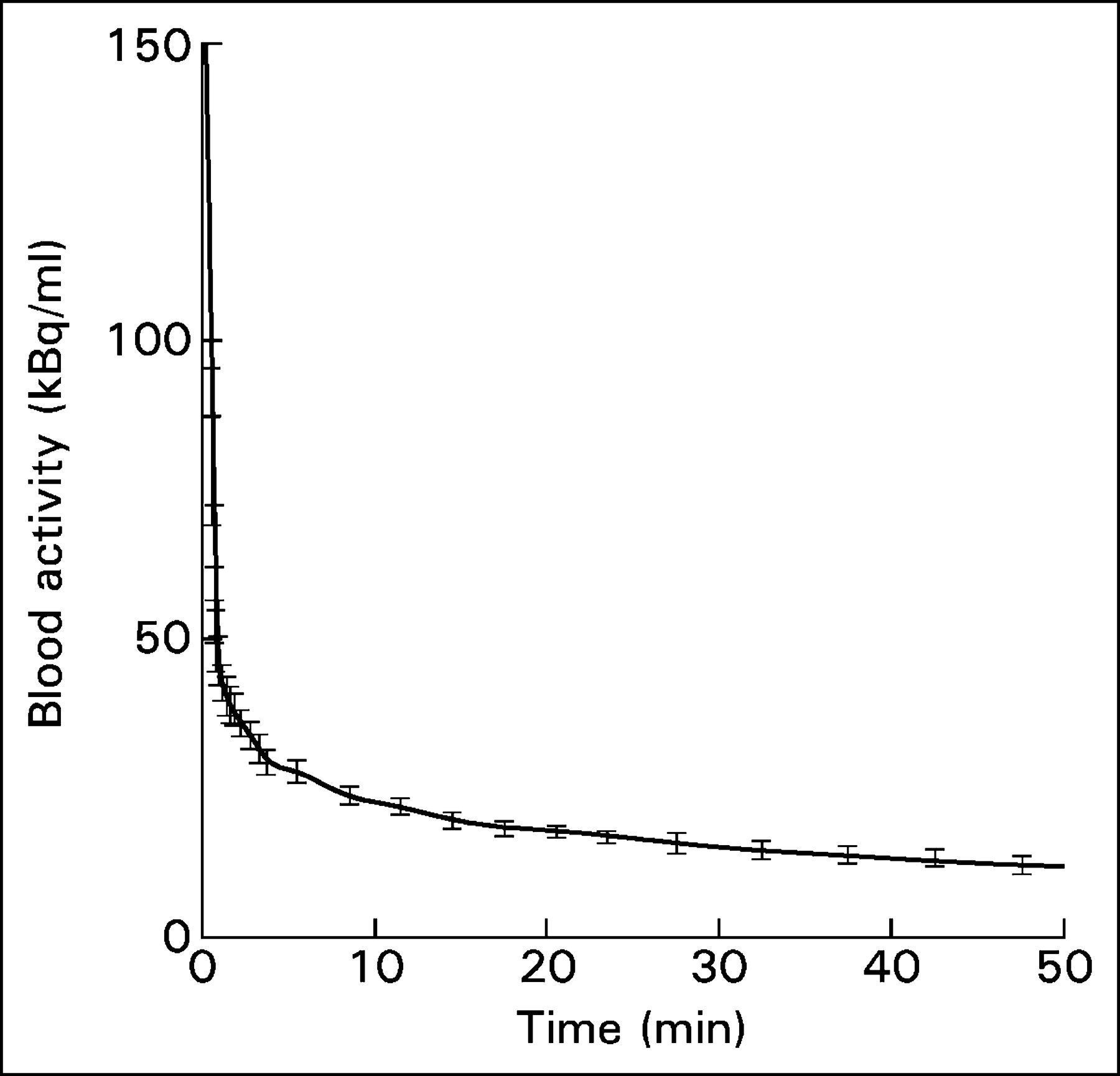
The input functions from the 18 subjects in population B were temporally aligned (by extrapolating the maximum up-slope of the bolus arrival to the time of zero activity) and averaged to obtain an average population input function (input function B), as shown in Figure 1. The error bars in Figure 1 represent the SE of the left atrial activity across the 18 subjects. As another rough indicator of the variability of the input function, we computed 0∫TA(t) (the primary determinant of the Patlak slope) at each time point T for each of the 18 subjects of population B and correlated it with the same quantity from a scaled population average made up of the other 17 subjects. The average SD of the individual input functions was 3% (range, 1%–6.2%).

Population input function generated by averaging the input functions from the 18 subjects in population B. The error bars represent the SE of blood activity across all patients.
Patlak Analysis.
Standard Patlak analysis was performed on population A using each patient’s individual input function and tumor time-activity curve. The data from 10 min (to allow for equilibration) to the end of acquisition were used to obtain the slope Ki and intercept Vd (the 18F-FDG volume of distribution) of the Patlak plot, as well as to determine the estimated errors in those 2 parameters. All computations and weighted linear regressions were performed using IDL (Research Systems Inc.).
SKA-S Method.
The SKA-S method has been described in detail by Hunter et al. (5). The SKA-S method normalizes 18F-FDG uptake in the tumor to an estimated integral of the input function up to the time of the static scan. Hunter found that in nondiabetic subjects, the input function could be approximated by 3 decaying exponentials and that the 2 early exponents had minimal variation. Hence, any interpatient variability in the input function was attributed to the late part of the curve. The magnitude of the late part of the curve (the amplitude of the third exponent) was determined from a single late venous sample. Thus, in the SKA-S method, the integral is estimated using a combination of a triexponential function and a late venous sample, as specified by Hunter et al. (5). The resulting estimated integral is then used to normalize the 18F-FDG uptake in the tumor. This normalized uptake, which we call SKA-S, has been shown to be an approximation to Ki.
SKA-M Method.
The hybrid method proposed here (SKA-M) is illustrated in Figure 2. It combines some of the ideas of SKA-S and other previous methods (4–9) with Patlak analysis. We applied SKA-M to either late 1-level studies, using all the data from 25 to ∼55 min; late 2-level studies, using every other data point from 25 to ∼55 min; or 3-level studies, using every third data point between 10 and 55 min. We refer to these as 1-level SKA-M, 2-level SKA-M, and 3-level SKA-M. The concept of doing a dynamic, multilevel scan, alternating between levels, was described in the abstract of Hoh et al. (10). The input function for our SKA-M calculations was obtained by scaling the population-based input function to the patient’s own blood activity concentration at 40 min. This measurement is easily obtained either from a venous blood sample or from the image data (when the heart is in the field of view). In the latter case, to reduce noise, we smoothed the dynamic blood-pool time-activity curve from 25 to 55 min by fitting it to a biexponential function. The 40-min blood data were extracted from this fitted curve. The scaling factor was then calculated as follows:
 Eq. 1
Eq. 1

Illustration of SKA-M for 1 field of view. Both axes are similar to regular Patlak analysis except that a population input function, Apop(t), is used for A(t). Ameas(t) is determined as in Equation 2. One-level SKA-M requires only a few late time points (in this case between 25 and 55 min after injection). The regular Patlak analysis requires a full dynamic acquisition from the time of injection to about 60 min. Two-level SKA-M uses only every other point at each field of view, whereas 3-level SKA-M uses every third point from 10 min to ∼55 min (not shown).
The population input function was then scaled by the scaling factor and a Patlak analysis was performed using the dynamic tumor data and the scaled population input function. Dynamic data to determine SKA-M were either all data between 25 and 55 min (6–7 time points over 1 field of view), called 1-level SKA-M; every other data point between 25 and 55 min (the data available if 2 fields of view were to be imaged), called 2-level SKA-M; or every third data point from 10 to 55 min (leaving time to image 2 additional levels, if desired), called 3-level SKA-M. That is, by assuming that the scaled population input function is an accurate estimator of A(t), then:
 Eq. 2 where tumor(t) is the measured tumor tissue activity curve, Apop(τ) is the arterial curve as determined from the scaled population average curve, the integral is from 0 to time t, and Ameas(t) is the blood concentration determined at the times corresponding to the tumor points (e.g., a few points from 25 to 55 min).
A straight line was fit to the plot of tumor(t)/Ameas(t) versus {∫0tApop(τ)}/Ameas(t). The slope of this line is an estimate of Ki, which we call SKA-M, and the intercept of the line is an estimate of Vd, the fraction of unmetabolized 18F-FDG. The SKA-M value differs from Ki in 2 ways: First, instead of using a patient’s own input function, a scaled population input function is used. This results in a smoother input function and avoids the need for acquiring an input function for each subject. Second, Equation 1 requires only tumor data from 25 min (or later) to ∼55 min for 1-level imaging, and tumor data are needed from only every other or every third point for imaging 2 or 3 levels.
Statistical Analysis
The P value given for all correlation coefficients indicates the probability that the correlation coefficients differed significantly from zero. Comparisons of variance were performed using the F distribution. Slopes and intercepts were determined from linear least-squares regression analysis. SKA values were compared with Patlak values using the Student t distribution, unpaired, except where indicated.
RESULTS
Comparison of SKA Methods and Patlak Analysis
Figure 3A shows the correlation between individual SKA-S values and the Patlak slope. SKA-S was computed using Hunter’s published values for the 3 fixed parameters and using each subject’s blood activity at 40 min. Figures 3B and 3C show the correlation between the individual values of the Patlak slope and SKA-M, for 1 level (i.e., using all data from 25 min to ∼55 min) and for 3 levels (i.e., using only every third datum point from 10 min to ∼55 min), respectively. SKA-M was estimated using the population-B input function, scaled by each subject’s 40-min blood sample. Both SKA-M and SKA-S correlated well with Patlak slope (r > 0.99, P < 0.001, for both 1- and 3-level SKA-M and r = 0.96, P < 0.001, for SKA-S). The data scattered more widely about the regression line with SKA-S than with either 1- or 3-level SKA-M (12.9% for SKA-S vs. 1- and 3-level SKA-M values of 3.5% and 4.6%, respectively; P < 0.01). The SKA-S regression line (Fig. 3A) had a slope considerably different from unity and a positive intercept. Both SKA-M regression lines were closer to unity and had a negligible intercept. A similar good correlation was found when only every other point of the 25- to 55-min data was used, as would be required for a 2-level study (r > 0.99, slope = 0.93, and intercept = 0.0012, with a scatter of 4.4% about the regression line).
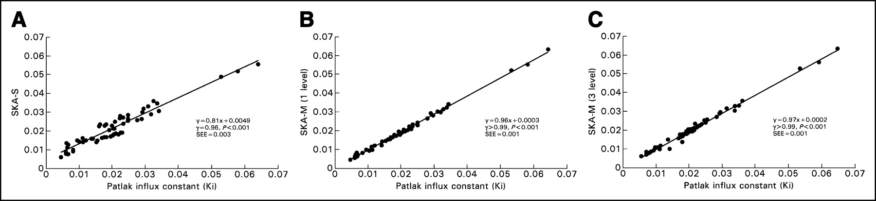
(A) Correlation between SKA-S (mL/g/min) and Ki (mL/g/min), along with the regression line. (B) Correlation between 1-level SKA-M (mL/g/min) and Ki (mL/g/min), along with the regression line. Visually, the scatter appears to be larger in the SKA-S plot than in the SKA-M plot. The SD of the data about the line was 3.5% for 1-level SKA-M and 12.9% for SKA-S (P < 0.01). (C) Correlation between 3-level SKA-M (mL/g/min) and Ki (mL/g/min), along with the regression line. There is less variability about the regression line (4.6%) for 3-level SKA-M than for SKA-S (P < 0.05).
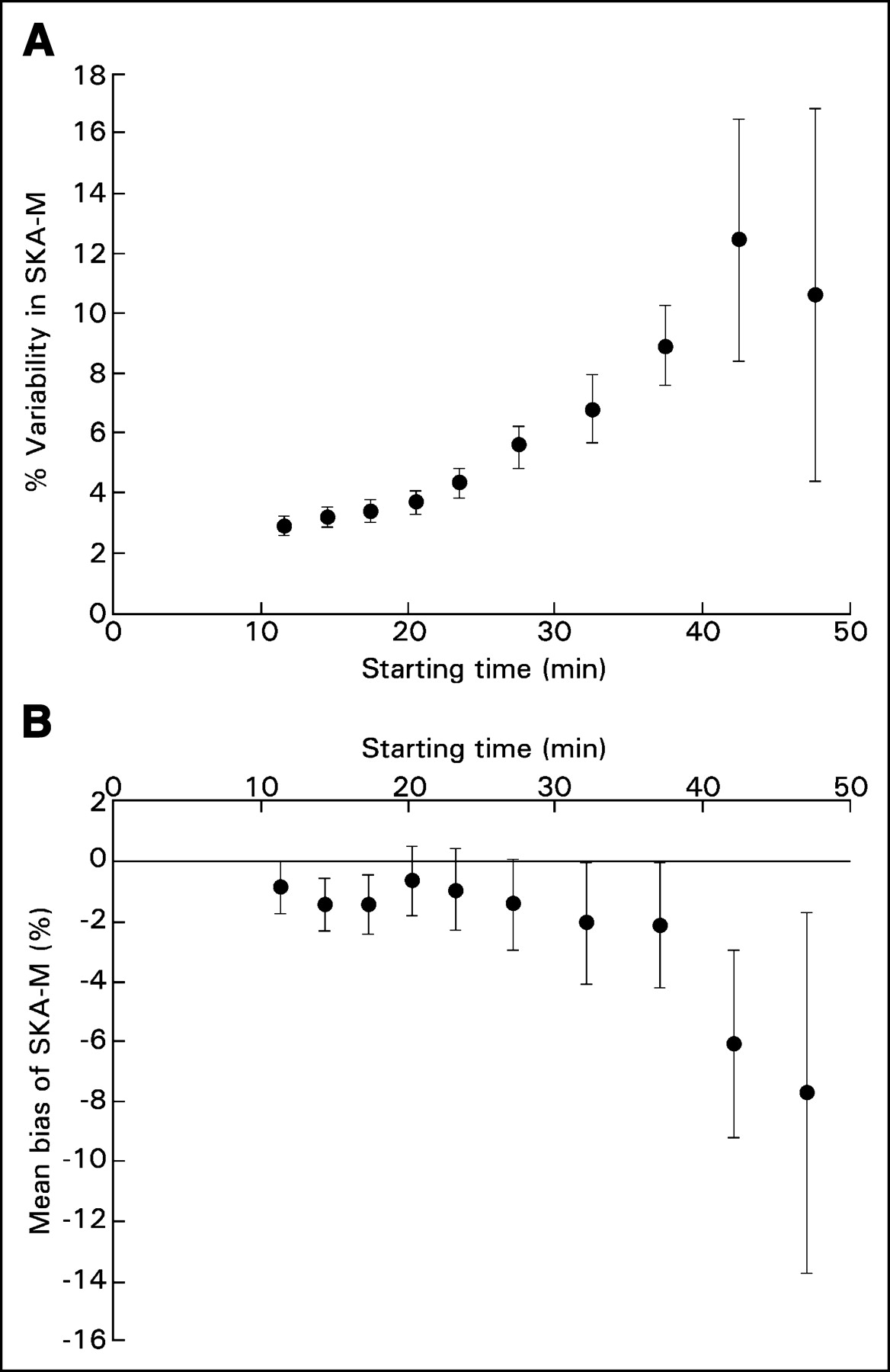
Because SKA-M uses fewer time points in the fit than does full Patlak analysis, the slope estimates for SKA-M may have increased statistical error. It was hoped that this increase would be partially offset by the reduced statistical fluctuations inherent in using a population-based input function. To determine whether this was true, we compared the estimated SD of the slope of each fit obtained using SKA-M with that obtained using true Patlak analysis. The average of each of these percentage SDs in the Patlak slope (full Patlak analysis with starting time of 10 min for the Patlak fit) was 5.7%, whereas it was 4.3% for 1-level SKA-M (P = not statistically significant), 6% for 2-level SKA-M, and 9.1% for 3-level SKA-M (neither significantly different from the SD for full Patlak). Figure 4A shows how the statistical fluctuations in computing the slope by 1-level SKA-M increase as the number of time points is reduced, keeping the ending time constant.

(A) Effect on SKA-M variability of changing the starting time for the SKA-M fit. The variability of SKA-M progressively increases as later starting times are used. (B) The effect on percentage difference between Ki and SKA-M of changing the starting time for SKA-M. Delaying the starting time for SKA-M results in progressively larger differences between SKA-M and Ki (mean bias of SKA-M).
We also investigated whether using fewer time points could introduce a bias between SKA-M and Patlak. Figure 4B plots the observed percentage bias, 100 × (SKA-M - Ki)/Ki, versus the starting time (1-level data). Bias slowly increased from about −1% at the 25-min start time to ∼−2% at 37 min. At later times, bias increased further. Both 1-level SKA-M and SKA-S were found to be statistically significantly different from Patlak analysis (P < 0.01 for SKA-M and P < 0.04 for SKA-S by paired analysis). However, 1-level SKA-M differed from Ki by only −1.0% ± 1.4%, whereas SKA-S differed from Ki by 15.1% ± 3.9%.
Comparison of SKA Methods and Patlak Analysis in Individual Patients
The results describe the average behavior of SKA-S and SKA-M over all subjects. We also calculated the number of tumors in which a given SKA method would differ from Patlak analysis by more than 20% (twice the SD previously reported for reproducibility of SUVs and Patlak values (12)). With 1-level SKA-M, tumors in only 2 of 27 studies differed from Patlak by more than 20%, whereas with SKA-S, tumors in 10 of 27 studies differed by more than 20% from Patlak (P < 0.02 by χ2 analysis). Fewer studies disagreed with Patlak using SKA-M than using SKA-S, presumably because of the smaller slope and positive intercept of the SKA-S regression line, as well as the increased variability of SKA-S about its regression line.
DISCUSSION
Patlak analysis and compartmental analysis are generally considered gold-standard methods for evaluation of tumor glucose metabolism but are cumbersome to use. Using the SUV is far simpler and more practical but is known to have at least 2 major deficiencies. First, it does not account for physiologic changes in the available dose to the tumor (i.e., it does not correct for variations in the integral of the input function). Second, SUV is the sum of the 18F-FDG that has been metabolized and trapped by the tumor cells plus the free 18F-FDG, which has not been metabolized and is in the intravascular, interstitial and unmetabolized intracellular compartments. If images could be acquired at very late times (e.g., many hours after injection), it is possible that the second of these deficiencies could be made negligible (13), but late acquisition is often impractical. SKA methods attempt to overcome some of the limitations of the SUV. The method of Hunter et al. (5), which we refer to as SKA-S, is one such method. By using a standardized functional form for the input function, based on a population average, and by taking a single late venous blood sample, SKA-S attempts to compensate for potential changes in the integral of the input function (the available dose). However, because SKA-S does not follow tumor uptake dynamically, it does not correct for unmetabolized 18F-FDG. The unmetabolized 18F-FDG fraction has been estimated to vary from 6% to 67% (14). Hence, the unmetabolized free 18F-FDG fraction is often a considerable and variable fraction of uptake in the tumor, even 50–60 min after injection. The SKA-M method proposed here tries to combine some of the advantages of SKA-S with the accuracy of the Patlak method. The SKA-M 1-level method uses a few dynamic images acquired late (e.g., beginning 25 min or later after injection) to monitor the rate of uptake of 18F-FDG by the tumor. SKA-M is a modified Patlak analysis in which the input function from the individual patient no longer has to be measured and instead is replaced with a single population-averaged input function, scaled with a late blood sample. It was hypothesized that by combining late dynamic imaging with a scaled population input function, SKA-M could correct for both available dose and unmetabolized 18F-FDG and so would agree better with Patlak analysis.
We found that SKA-S correlated well with Patlak analysis (r = 0.96), in agreement with the findings of Hunter et al. The scatter of the SKA-S values about the regression line was somewhat higher than that found for SKA-M (12.9% vs. 4%–5%). In addition, the slope of the SKA-S regression line differed significantly from unity (slope = 0.807), with a significant intercept (0.0049, or 23.3% of the mean value). In contrast, the SKA-M method for 1, 2, or 3 levels had slopes closer to unity (>0.930) and an intercept closer to zero (<0.0007, or <3.7% of the mean). The positive intercept and nonunity slope resulted in a bias of SKA-S compared with Ki of about 15% (range, −18% to 113%), versus a bias of about 1% for SKA-M. Because of this bias, SKA-S differed from Ki by greater than 20% in 10 of 27 studies. The SKA-M 1-level method differed from Ki by greater than 20% in only 2 of 27 studies. We speculate that these differences occurred because SKA-S does not correct for unmetabolized 18F-FDG, whereas SKA-M does.
One might speculate that the bias (but not the variability) in SKA-S could be nearly eliminated by knowledge of the regression line. However, if the presence of unmetabolized 18F-FDG is indeed part of the reason for the low slope and positive intercept of the regression line, then the regression line might well be different for subjects with different amounts of unmetabolized 18F-FDG (e.g., subjects with inflammatory processes). When tumors have low metabolic activity, even a small amount of unmetabolized 18F-FDG becomes a significant fraction of total 18F-FDG uptake in the tumor. For example, we found that SKA-S differed, on average, from Ki by 45% ± 7.3% when Ki was less than 0.015 mL/g/min but by only 1.7% ± 2.5% when Ki was more than 0.015 mL/g/min. On the other hand, the SKA-M 1-level method differed from Ki by 7% ± 3.5% when Ki was less than 0.015 mL/g/min and by −4.7% ± 0.7% when Ki was more than 0.015 mL/g/min. Hence, for tumors with low uptake, neglecting the unmetabolized 18F-FDG concentration may cause large percentage errors in SKA-S. SKA-M may be particularly useful in this situation. Conversely, if our patient population had contained fewer tumors with low uptake (e.g., <0.015 mL/g/min), SKA-S may have had a lower percentage disagreement with Patlak analysis.
The values of SUV, and to a lesser extent SKA-S, depend on the time at which imaging is performed. At the usual acquisition time of around 60 min after injection, many tumors have not reached their uptake plateau. Reaching the plateau has been found to take as long as 256–340 min after injection for many tumors (2,13). SKA-M in theory does not depend on the time of imaging because it is a measure of rate of uptake rather than uptake at a specific time. This is confirmed in part by the data in Figure 4B, although there was a small (statistically insignificant) increase in bias at very late times (presumably because of the very small number of points used). We speculate that if very late static images were used, both SKA-S and SKA-M might have agreed equally well with Patlak analysis (with SKA-S being simpler to implement).
In summary, both SKA-M and SKA-S correlated well with Patlak analysis. SKA-M had less variability about the regression line, a regression slope closer to unity, and no significant intercept. In addition, because SKA-M follows the rate of uptake, it can account for unmetabolized 18F-FDG, which may explain the smaller bias (1% vs. 15%) compared with SKA-S. By measuring rate of uptake, SKA-M, in principle, removes the dependence on uptake time that SUV exhibits. The SKA-M 1-level method reduces imaging time by more than 40% and, equally important, avoids the necessity of measuring the input function. A wide range of studies has investigated the therapeutic efficacy of new drugs. Many of these studies follow one or more index tumors in a single organ, as a function of time. The SKA-M 1-level or 2-level method would be well suited to such studies. The small variability in uptake slope determined with SKA-M, even when dynamic imaging is delayed further than 25 min (Fig. 4A), is presumably due to the smoothness of the population-based input function. This possibility, combined with the relatively low bias as a function of time (Fig. 4B), suggests that imaging could be delayed still more, further shortening the acquisition.
We did not attempt to validate the SKA methods using clinical criteria such as survival, time to disease progression, or change in CT tumor size with treatment. Our aim was to develop and validate a simple measure of the glucose metabolic rate of the tumors with only a limited dynamic acquisition. Hence, in this context, we selected the influx constant obtained using a regular Patlak analysis as our gold standard for validating the SKA methods.
A potentially significant drawback of SKA-M is that it requires a longer imaging time than does SKA-S, although conceivably, from Figure 4, this imaging time could be reduced. Finally, although our subjects had a wide range of blood glucose levels, it remains to be seen whether a population average is adequate for characterizing subjects with a drastically altered overall glucose metabolism, as in diabetes. This is also true for most SKA methods.
CONCLUSION
Both SKA-M and the SKA-S compared well with Patlak analysis. In the population studied, SKA-M had lower variability and less bias than did SKA-S, compared with Patlak analysis. We speculated that the reason was the ability of SKA-M to correct for unmetabolized 18F-FDG by monitoring tumor uptake dynamically, whereas SKA-S could not. This correction appeared especially significant in tumors with low 18F-FDG uptake rates and could be important in any tumor with large unmetabolized pools of 18F-FDG, as might occur in inflammatory processes or in nonviable regions of tumor. In such situations, SKA-M may be preferred over SUV or other methods such as SKA-S that do not follow the dynamic course of tumor uptake.
Footnotes
Received Aug. 14, 2003; revision accepted Dec. 8, 2003.
For correspondence or reprints contact: Stephen L. Bacharach, PhD, Bldg. 10, Room 1C401, NIH, Bethesda, MD 20892-1180.
E-mail: steve-bacharach{at}nih.gov
REFERENCES


Jump to section
Related Articles
Cited By...
- Is Liver SUV Stable over Time in 18F-FDG PET Imaging?
- Searching for Alternatives to Full Kinetic Analysis in 18F-FDG PET: An Extension of the Simplified Kinetic Analysis Method
- Is the Physical Decay Correction of the 18F-FDG Input Function in Dynamic PET Imaging Justified?
- Image-Derived Input Function for Assessment of 18F-FDG Uptake by the Inflamed Lung
- Partial-Volume Effect in PET Tumor Imaging
- Consensus Recommendations for the Use of 18F-FDG PET as an Indicator of Therapeutic Response in Patients in National Cancer Institute Trials