


Abstract
Nuclear medicine renal studies can be performed using slow-rotation SPECT, but reconstruction of such data is largely underdetermined. Methods: A new method of reconstruction of data acquired using slow camera rotations was developed. In this method we used a factor model of the data in which the factors and factor coefficients were determined by modeling their relationship directly with the projection measurements. This was done by solving a least-squares problem that fits the projections of factors and factor coefficients to the projection data with nonnegativity constraints imposed on the solution. The method was tested on computer simulations and applied to experimental renal 99mTc-mercaptoacetyltriglycine canine and patient studies. Results: Computer simulations showed that the extracted time–activity curves of kidneys agreed well with the simulated curves for data with noise levels similar to those in the experimental studies. In the canine study, the method showed that >2 factors were necessary to adequately reproduce the kinetics of the kidney. In the patient study, the method was able to extract separate factors that correspond to the kidney cortex and the kidney pelvis. Conclusion: The computer simulation, the canine study, and the patient study all show that reconstructions of the data obtained with 1 detector displayed artifacts, whereas reconstructions of the data obtained with 2 and 3 detectors were free of artifacts. Computer simulations showed that the method gives accurate results that allow quantitation.
Nuclear medicine renal studies are performed by measuring the clearance of radiopharmaceuticals from the kidneys to determine kidney performance. One of the common agents used in these studies is 99mTc-mercaptoacetyltriglycyne (MAG3), which offers major advantages in clinical use over other agents because it provides a better target-to-background ratio and, thus, a better contrast in the acquired images (1).
Dynamic studies are used to measure the 99mTc-MAG3 kinetics in the kidneys. The most common method of dynamic data acquisition is a planar study. After the data acquisition, regions of interest (ROIs) are drawn on the acquired images, and the time behavior of the summed counts in these regions is obtained. The relation between counts in a given ROI versus time generates a time–activity curve. The time–activity curves can also be extracted automatically from a series of dynamic planar images by using factor analysis of dynamic structures (FADS) (2).
A disadvantage of the planar data acquisition is that the counts from different organs may be superimposed. As a result, time–activity curves from ROI measurements represent the time behavior of the sum of the activities from these organs. The results obtained with FADS in planar renal imaging are not unique because of the complete overlap of the kidney with the background (3). Also, planar imaging does not provide quantitative results because accurate correction for photon attenuation cannot be performed.
Quantitation in renal studies is important. One of the applications of quantitative renal imaging is calculation of the glomerular filtration rate (GFR), which is an important indication of kidney function. The GFR is most accurately calculated using invasive blood sampling. The GFR can also be calculated from radiographic planar studies; however, because of a lack of accurate quantitation in the radiographic studies, the GFRs calculated this way are not accurate.
To overcome these limitations, SPECT techniques have been investigated for use in dynamic cardiac studies (4). The tomographic acquisition protocol of the dynamic data can be based on either fast or slow camera rotations. In fast-rotation acquisition, a complete set of tomographic data is acquired over a very short period of time (approximately 10 s) resulting in low count projections and noisy images in the reconstructed series.
In this investigation we used a slow-rotation approach to dynamic data acquisition. During the acquisition the camera rotates slowly around the object. Such acquisition is similar to that of a standard static acquisition of SPECT data. Only a small number of rotations of the camera are made during the scan (5–10).
Various methods in PET and SPECT have been used to estimate parameters of kinetic models directly from projections (11–19). These methods can also be used with the slow-rotation acquisition. However, all of these methods are based on an assumed kinetic model that governs the changes of the radiopharmaceutical in the object. Some methods require simultaneous reconstruction of tomographic images acquired by fast rotation to estimate the object boundary (15,16). Other methods estimate an initial set of exponential factors through eigenvalue analysis of projected dynamic sequences (17).
In this article we describe a technique that does not require any kinetic model but, rather, reconstructs a sequence of dynamic images from these inconsistent projections using a factor model of the dynamic physiologic images (20). In this method, each reconstructed dynamic image corresponds in time to 1 camera stop, unlike in the fast-rotation method in which 1 dynamic image corresponds to a full tomographic set of projections.
We present the theory and the results of the tomographic factor reconstruction method using data from a computer simulation of renal uptake of a radiopharmaceutical. The method was also applied to experimental 99mTc-MAG3 canine and patient studies.
MATERIALS AND METHODS
Objective Function
The counts in the projection bin j taken at the time t, Pj(t), are expressed by the following projection equation:
 Eq. 1
Eq. 1
The value of αji(t) is an element of a system matrix. The symbol i is an index of the pixel in the dynamic image A, and Ai(t) represents the activity in pixel i at time t. Coefficient αji(t) is proportional to the probability that the photon emitted from pixel i at time t is detected in bin j of the projection taken at time t. N is the number of pixels in the image. It is assumed in Equation 1 that the activity in the object remains constant during the measurement of each projection.
A can be estimated by constructing and minimizing a weighted least-square objective function:
 Eq. 2
Eq. 2
The value of P̂j(t) is the experimental value of counts in the j-th projection bin collected at the projection taken at time t. M is the number of bins in the projections and K is the number of projections.
The solution to Equation 1, which is obtained through optimization of Equation 2, is largely underdetermined. The number of unknowns is approximately 100 times higher than the number of equations. The solution of Equation 1, without constraints, corresponds to the reconstruction of an image at each time point from only 1 projection when 1 detector is used or from 3 projections when 3 detectors are used for the acquisition.
To reduce the number of unknowns, the factor model of the data is used. This means that each image is built from groups of pixels that have the same temporal behavior (21). Mathematically this can be expressed by:
 Eq. 3
where Cis is the value of the s-th factor coefficient for pixel i and Fs(t) is the value of the s-th factor at time t. Usually, as in the FADS method, the number of these groups (number of factors S) is equal to the number of physiologic factors—that is, factors actually present in the medical image. However, in the method presented in this article, the number of factors was not restricted to the number of physiologic factors (20). Using the factor model, the number of unknowns is equal to S(K + N), which is substantially lower than the initial KN number of unknowns. For renal studies S is usually equal to 2 or 3. Although the number of unknowns is reduced by introducing the factor model, it also causes the objective function Equation 2 to be nonlinear. Using Equations 2 and 3, the objective function becomes:
Eq. 3
where Cis is the value of the s-th factor coefficient for pixel i and Fs(t) is the value of the s-th factor at time t. Usually, as in the FADS method, the number of these groups (number of factors S) is equal to the number of physiologic factors—that is, factors actually present in the medical image. However, in the method presented in this article, the number of factors was not restricted to the number of physiologic factors (20). Using the factor model, the number of unknowns is equal to S(K + N), which is substantially lower than the initial KN number of unknowns. For renal studies S is usually equal to 2 or 3. Although the number of unknowns is reduced by introducing the factor model, it also causes the objective function Equation 2 to be nonlinear. Using Equations 2 and 3, the objective function becomes:
 Eq. 4
Eq. 4
To ensure the nonnegativity of the resulting matrix A, nonnegativity constraints are imposed by adding the term fneg(C, F) to the objective function:
 Eq. 5
where
Eq. 5
where
 with a being a penalty constant. Although the results presented in this article are for a 2-dimensional (2D) case, all equations are also valid for a 3-dimensional (3D) case.
The minimization of Equation 4 yields optimal values of C and F, which usually are not physiologically meaningful—that is, images of the factor coefficients may not correlate with physiologic regions and factors may be substantially different than the real-time behavior of the pharmaceutical uptake and washout in organs. Matrices C and F are not physiologically meaningful because (a) in general, the value of S is different than the number of physiologic true factors present in the image, and (b) matrices C and F, which result from the minimization, are not mathematically unique. This nonuniqueness of the tomographic factor analysis solution is similar to the nonuniqueness of FADS discussed elsewhere (22,23). The dynamic sequence A obtained using Equation 3 is the final result of the method.
The data were processed on a SUN SPARC ULTRA 60 (Sun Microsystems, Inc., Mountain View, CA). Each reconstruction required approximately 20 h of computing time per slice. The same starting point was chosen for all of the optimizations. The matrix C was initiated with a constant value of 0.1. Initial factors were linear functions of time. The initial values of the CF matrix were approximately 10. The conjugate gradient (24) method was usedfor the optimization. Iterations were terminated when the relative change in the objective function was <10−6.
Computer Simulations
Computer simulations were performed to verify the validity of the reconstruction methods. Uptake of the radiopharmaceutical in the cortex of the kidney was simulated by the following function:
 where A = (1 − exp[−0.693td/T½ ]). Time in Equation 7 was represented by t, td was the delay time introduced by the cortex, T½ was the half-life of the biologic clearance from the kidney, and I was a scaling factor. The background activity b(t) was simulated as the exponential decrease of (Fig. 1):
 Eq. 8
with IB being a scaling constant for the background and ½B being the half-life of the clearance of the activity from the background. The shapes of the kidneys were simulated as ellipses (Fig. 2A), and the activities in the left kidney (LK) and the right kidney (RK) were simulated using Equation 7. For the LK parameters, I was equal to 80; td and T½ were 220 and 400 s, respectively. For the RK, the same time parameters were used and I was equal to 100. The background was assumed to be uniform, and the amplitude IB in the left portion of the body background (LB) (Fig. 2A) was 1 and the amplitude for the right body background (RB) was 2. The value of ½B was 1,600 s. All of the above values were chosen to approximate the time behavior of the curves observed experimentally in renal studies. The above equations were derived from earlier work (25).
Eq. 8
with IB being a scaling constant for the background and ½B being the half-life of the clearance of the activity from the background. The shapes of the kidneys were simulated as ellipses (Fig. 2A), and the activities in the left kidney (LK) and the right kidney (RK) were simulated using Equation 7. For the LK parameters, I was equal to 80; td and T½ were 220 and 400 s, respectively. For the RK, the same time parameters were used and I was equal to 100. The background was assumed to be uniform, and the amplitude IB in the left portion of the body background (LB) (Fig. 2A) was 1 and the amplitude for the right body background (RB) was 2. The value of ½B was 1,600 s. All of the above values were chosen to approximate the time behavior of the curves observed experimentally in renal studies. The above equations were derived from earlier work (25).

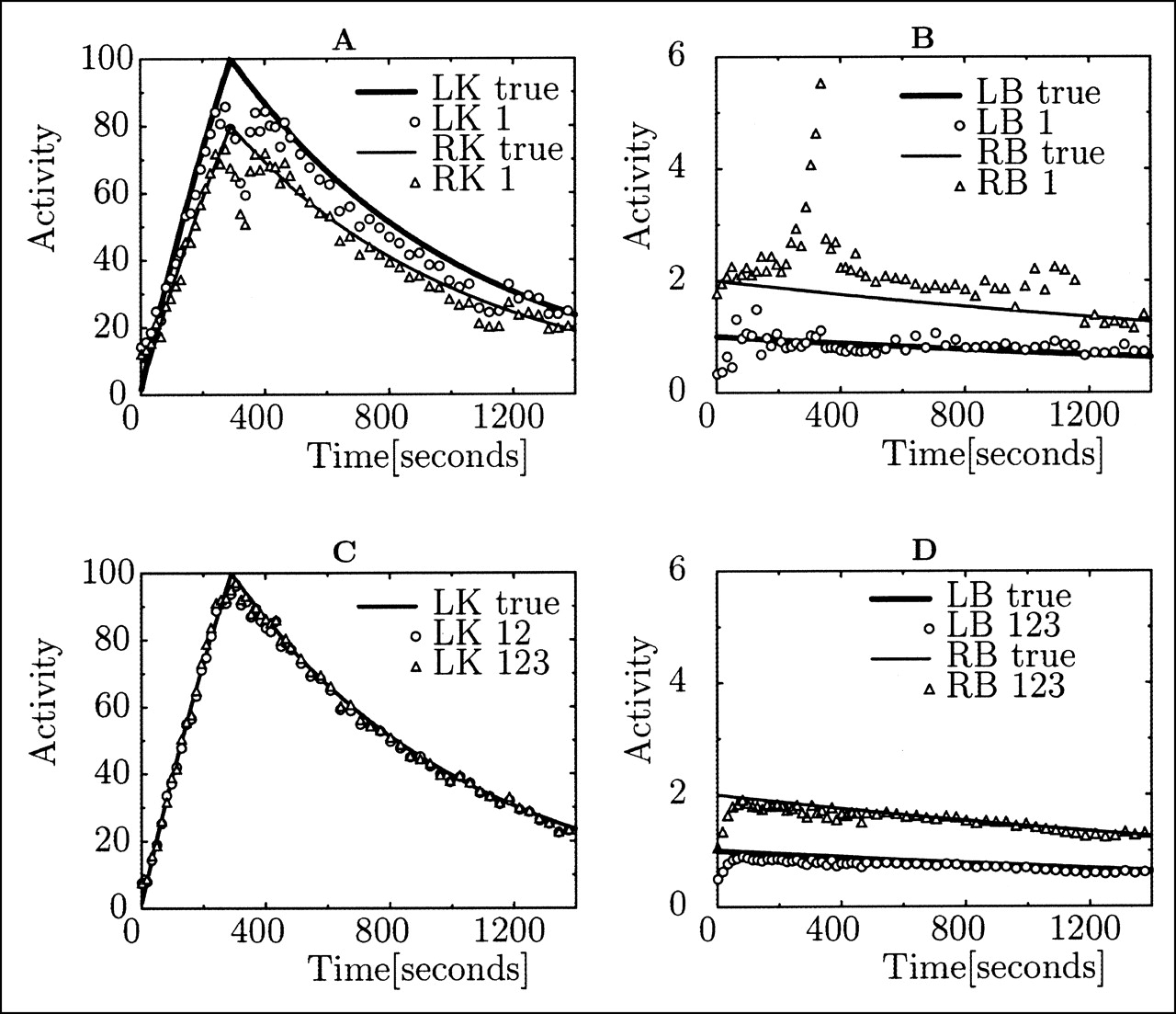
Comparison of true time–activity curves and curves obtained from reconstructions of left and right kidneys (LK and RK, respectively) (A) and backgrounds (LB and RB, respectively) (B). (A and B) Kidney and background time–activity curves were obtained using only detector 1 (Fig. 3A). (C and D) Time–activity curves of LK and background obtained with >1 detector. Number 1, 2, or 3 indicates which detector was used in reconstruction. Only every third time point is shown when symbols are used.
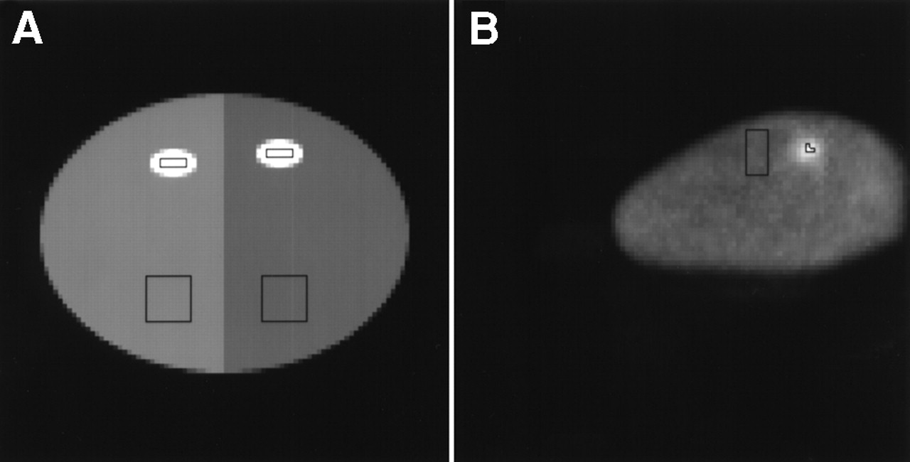
(A) Phantom used in computer simulations. Bright small ellipses correspond to simulated kidneys. Large ellipse representing body outline is divided into left body background (LB) and right body background (RB), which have different intensity levels (shown as different shades). Rectangles encompass ROIs used for time–activity curve extractions. (B) Image of left kidney (LK) in canine study superimposed on attenuation map approximately 4 min after injection. Rectangular regions correspond to ROIs used for extraction of time–activity curves of LK (small 3-pixel ROI) and background (large 50-pixel ROI). Dog was positioned off-center during experiment.
Another set of computer simulations was performed to simulate abnormal uptake in the RK and the normal uptake described by Equation 7 in the LK. The abnormal uptake nab(t) was assumed to be an asymptotic increase of activity in the kidney and was described by the following equation:
 Eq. 9
Eq. 9
Projections of the 2D phantom were then generated. Each projection had 128 bins and a total of 120 projections was taken. A 3-head detector acquisition was simulated with the heads positioned 120° apart (Fig. 3A). The first 60 projections were taken for 8 s each over a 180° clockwise rotation of the camera, and the other 60 projections were taken for 16 s each over a 180° counterclockwise rotation starting from the end position of the first phase of the acquisition. Uniform attenuation throughout the object was simulated with an attenuation coefficient equal to 0.15 cm−1. A perfect parallel-hole collimator was assumed, and scatter and collimator blurring were not included in the simulations. Poisson noise was added to simulate noisy data. Two levels of noise were simulated. The total number of counts per head per slice during the entire study was equal to 220 and 110 kilocounts (kcts). For the normal study, in which both kidneys were simulated using Equation 7, 3 simulations corresponding to 3 different noise levels (no noise, noise level 1, and noise level 2) were performed. The normal study consisted of a simulation with 2 physiologic factors with the activities in the pixels subject to change according to either Equation 7 or Equation 8. For the abnormal study, 3 simulations corresponding to the same 3 different levels of noise were also performed. The abnormal study corresponded to a simulation of 3 physiologic factors: normal uptake in the kidney, n(t); abnormal uptake in the kidney, nab(t); and activity in the background, b(t). Ten noise realizations were used. The number of heads used for the reconstructions and the number of factors S in Equation 4 were varied.

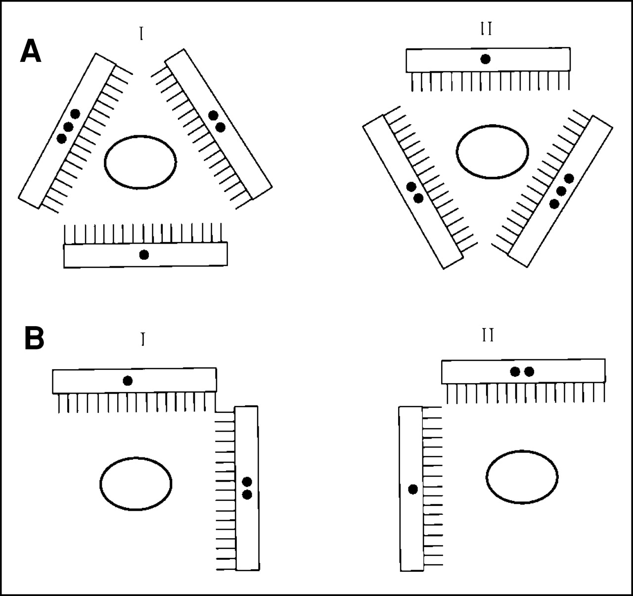
Diagram of acquisition protocols used in computer simulations (A) and experimental canine 99mTc-MAG3 renal study (A) and experimental patient 99mTc-MAG3 renal study (B). (A) In first phase of acquisition, 3-detector camera rotated from I to II in clockwise direction and acquired 60 projections for 8 s each over 180°. Camera was then returned to starting position (I) and, during second phase, it rotated in clockwise direction and acquired 60 projections for 16 s each over 180°. (B) For patient protocol, camera in first phase of acquisition rotated 90° clockwise and acquired 64 projections (from I to II). During second phase, it rotated back (from II to I) in counterclockwise direction and acquired 64 additional projections. Duration of all projections in patient study was 10 s. Number of dots indicates detector number.
The computer simulation study was divided into 3 phases. In the first phase, the results of studying the number of detectors in the acquisition were investigated. In the second phase, the effects of the number of factors used in the reconstruction were considered. In the third phase, the results of the reconstruction of the data with different levels of noise were obtained.
The number of reconstructed images equaled the number of projections; for the computer simulation, each image was 100 × 100 pixels. The kidney ROIs were rectangles of 6 × 2 pixels centered on the kidneys. The background ROIs were two 10 × 10 pixel squares positioned over the left and right parts of the phantom. These ROIs are presented in Figure 2A.
The accuracy of the reconstructions was assessed using the following error measure E:
 Eq. 10
where N̂(t) is a reconstructed time–activity curve that is an estimation of the true N(t).
Eq. 10
where N̂(t) is a reconstructed time–activity curve that is an estimation of the true N(t).
Canine Study
The canine study was performed using a 3-detector IRIX camera (Marconi Imaging Systems, Inc., Cleveland, OH). The camera was equipped with high-resolution, parallel-hole collimators. The tomographic study consisted of 2 phases (Fig. 3A). In the first phase, the 3-head camera rotated continuously over 180° acquiring 60 views per head (128 × 128 pixels) for 8 s each. It took 21 s for the camera to return to its initial position before the second phase started. In the second phase, which also acquired 60 projections over 180° in the same direction as the first phase, each view was acquired for 16 s. Approximately 1 h after the tomographic study, the planar study was performed; 180 views were acquired, each for 8 s. The radioactive bolus of 99mTc-MAG3 (333 MBq for SPECT and 407 MBq for planar study) was injected through an intravenous catheter placed in the left front leg of the 22.3-kg male dog at the same moment the acquisitions commenced. Data were acquired using a 15% energy window positioned at 140 keV. No scatter correction was performed.
Using our reconstruction method, 120 images, each comprising 100 × 100 pixels, were reconstructed and time–activity curves were determined for the selected ROIs. The kidney ROI spanned 3 pixels, which were determined as the pixels with the highest values of factor coefficients (matrix C) that corresponded to a kidney. A background ROI comprising a rectangle of 5 × 10 pixels positioned below the kidneys was chosen. The ROIs for the canine RK are marked in Figure 2B.
Before the emission acquisition, a transmission scan was obtained to acquire attenuation maps. Transmission scanning was performed using a 133Ba point source with an asymmetric cone-beam geometry (26). The maximum-likelihood expectation maximization algorithm was used for reconstruction of the attenuation maps. The attenuation maps were rescaled from the 356-keV energy to the 140-keV energy of 99mTc. Because the dog was not moved between the transmission and emission scans, no realignment between the attenuation maps and emission data was needed.
Patient Study
The patient study was performed using a 2-detector eCam camera (Siemens Medical Systems, Hoffman Estates, IL) equipped with high-resolution, parallel-hole collimators. For the tomographic study the detectors were positioned at a relative angle of 90° (Fig. 3B). As in the canine study, the acquisition consisted of 2 phases. During the first phase the camera was rotated 90° clockwise and acquired a total of 64 projections (128 × 128 pixels) for 10 s each. It took approximately 150 s for the camera to reset before phase 2 commenced. Phase 2 consisted of a rotation from the end position of the first phase, 90° counterclockwise. The patient was in a supine position during the acquisitions. A planar study was also performed, during which 300 views were acquired for 5 s each. The planar study was performed approximately 8 h before the tomographic study; therefore, the activity had almost completely decayed and washed out when the tomographic study was performed. The radioactive bolus of 370 MBq for SPECT and 37 MBq for the planar 99mTc-MAG3 study was injected into the left arm of the 40-y-old, 90-kg, healthy male patient at the same time the acquisitions commenced.
The attenuation maps were acquired simultaneously with the emission acquisition using a multiple line source transmission system (27). The values of the attenuation coefficients were rescaled from the value that corresponded to the 153Gd 100-keV energy to the value of the attenuation coefficient that corresponded to the 99mTc energy. No scatter correction was performed. Each reconstructed image was 88 × 88 pixels in size. The kidney ROI selected over the cortex comprised 3 pixels, and the procedure used to select the ROI was similar to the procedure used in the canine study. The kidney ROI sizes are small because the sizes of the kidneys in the transverse slices are small.
RESULTS
Results of Computer Simulations
Although projection data were simulated using 3 detectors, reconstructions using data from 1, 2, and 3 detectors were performed and the results were compared. In Figures 1A and 1B, the activity curves obtained from the reconstructions of the data taken with only 1 detector are presented. These curves are compared with the true curves of the LK and the RK (Fig. 1A), and for the LB and the RB (Fig. 1B). The results show some disagreement between the curves, which is attributed to the ambiguity of the reconstruction from projections using 1 detector. This ambiguity will be discussed later. Figures 1C and 1D present time–activity curves obtained for the LK and backgrounds using 2- and 3- detector reconstructions. The reconstructions with 2 and 3 detectors remove the ambiguity artifacts, and the estimated kidney time–activity curves are very similar to the true curves. Results presented in Table 1 show the presence of large errors when the reconstruction was performed using data from 1 detector and show a significant reduction in errors when 2 and 3 detectors were used in the reconstruction process. The number of factors used in the reconstruction (S in Eq. 4) varied from 2 to 5. The results of the simulations with different values of S are summarized in Table 1. We found that when increasing S the quality of the reconstructions was not affected with the exception of 1 case. In the abnormal case, a clear difference in accuracy can be seen between the reconstructions made with S = 3 and the reconstructions with S = 4 and S = 5.
Values of Curve Differences Obtained in Computer Simulations
The method successfully recovers the kidney time–activity curves at all noise levels when 2 or 3 detectors are used. Although the reconstructed activity curves of the kidneys are very accurate (the error given by the measure defined in Eq. 10 is approximately 5%), the background is reconstructed with much less accuracy, and for high noise levels the error was as high as 25%. However, for noiseless data the errors present in the kidney time–activity curves and the background time–activity curves were similar.
Results of Canine Study
The total number of counts in sinograms varied from 70 to 110 kcts depending on the detector head by which the data were collected. The anatomy of dogs is such that the kidneys are separated axially (Fig. 4A). As a result, only 1 kidney is present in any single slice. In the planar and tomographic studies we did not observe any differences in dynamic uptake and washout within the volume of the kidneys. Therefore, the kidneys were considered to be 1 dynamic component, which means that in the entire volume of the kidney the dynamics of the 99mTc-MAG3 was assumed to be the same. The validity of this assumption will be considered in the Discussion.
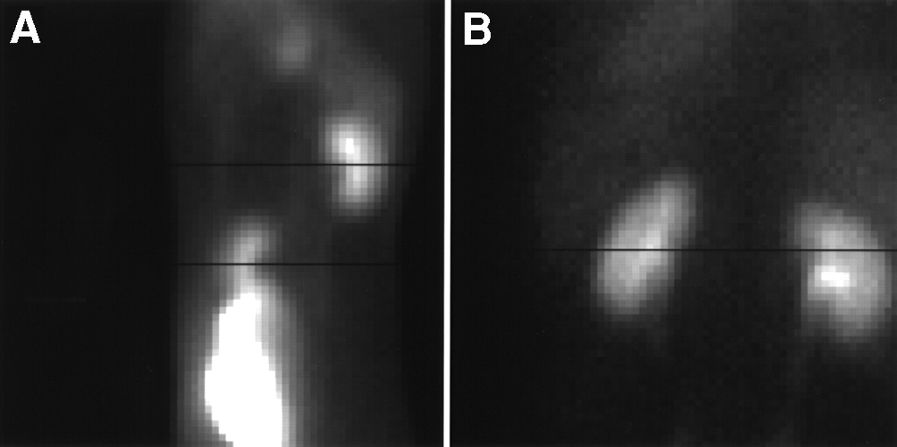
Summed images of planar studies for canine study (A) and for patient study (B). Black lines on images correspond approximately to slices that were reconstructed using SPECT.
Figure 5A shows the activity curves of the LK reconstructions using data from 1, 2, and 3 detectors. The results are similar to those obtained from the computer simulations. The reconstruction made with only 1 detector has artifacts in the kidney time–activity curves. The curves obtained from the reconstructions made using 2 and 3 detectors are similar and are free of artifacts.
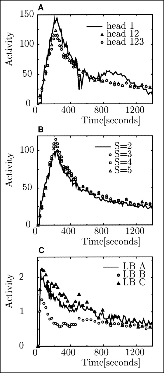
Time–activity curves obtained in canine study for LK. (A) Comparisons of reconstructions made with 1, 2, and 3 detectors. (B) Curves of LK derived from reconstructions made with 3-head camera with different values of parameter S. (C) Background curves reconstructed using data from 3 detectors (123) and with parameter S = 3; 3 curves correspond to 3 different ROIs. Only every third time point is shown when symbols are used.
The number of factors S in the objective function was varied in the reconstructions from 2 to 5. Results are presented in Figure 5B. There is little difference between the reconstructions made with 3, 4, and 5 components. However, they differ noticeably from the curve reconstructed with S = 2 because the factor model with S = 2 does not adequately describe all dynamic changes associated with the radiopharmaceutical uptake and washout that occurred in the canine study.
The background curves obtained from the projection reconstruction are presented in Figure 5C. It can be seen that these curves are inaccurate because it is expected that activity in the background decreases monotonically and the curves presented in Figure 5C do not. An image of the LK obtained 4 min after injection is presented in Figure 2B, in which the image of the LK in this figure is superimposed on the corresponding attenuation map. Results for the RK are not presented, but they are very similar to the results presented for the LK.
Results of Patient Study
In the reconstructed slice the total number of counts for detector head 1 was 130 kcts and for detector head 2 was 140 kcts. Examining the planar study, the dynamics of the uptake of 99mTc-MAG3 in the patient study varied in different parts of the kidney. Unlike the canine study, more components were required to describe the dynamic changes in the kidney. Two regions with different dynamics in the kidney were observed. One region corresponded spatially to the kidney cortex and the other region corresponded spatially to the kidney pelvis. The main temporal difference between these 2 regions was that the maximum activity in the cortex appeared earlier than did the maximum activity in the pelvis.
Figure 6 presents the results of the reconstruction of a slice that corresponds approximately to the slice marked in the results of the planar study in Figure 4B. The factors and factor coefficients presented in Figure 6 were obtained through the minimization of the objective function (Eq. 4). Because this slice contains the kidney pelvis of the LK (Fig. 4B), a distinctive factor is extracted. Its coefficient image corresponds spatially to the pelvis of the LK (Fig. 6C). The same slice does not contain the pelvis of the RK, so it is not visible in the coefficient image in Figure 6C.

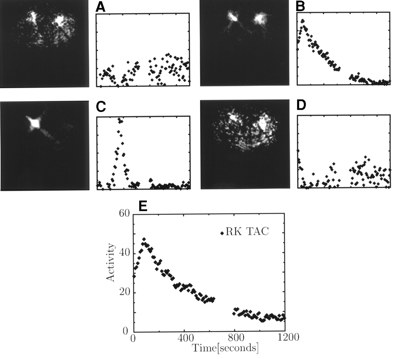
Reconstructed factors and factor coefficients of patient study. (A and D) Background. (B) Activity in kidney cortex. (C) Activity in kidney pelvis. (E) Time–activity curve (TAC) of RK, which is combination of A through D. Gap in data corresponds to time needed for detector configuration (Fig. 3B) to reset between phase 1 and phase 2 of acquisition.
Figure 6B presents the coefficient image that corresponds to the kidney cortex. The other 2 components in Figures 6A and 6D correspond to the background. As can be seen, factor coefficient images in Figure 6 correspond to the physiology of the kidney. The combination of 4 presented factors gives the time–activity curve of a desired region. The time–activity curve of the cortex for the RK (for which there is no pelvic component) is presented in Figure 6E. This time–activity curve is slightly different than the factor corresponding to the kidney cortex presented in Figure 6B.
DISCUSSION
In the reconstruction of the computer-simulated data, the projection and backprojection operations used to generate the data were the same as those used in the reconstruction. As a result, there was no mismatch between the system matrix used to create the data and the system matrix used in the reconstruction. Using these simulations it was shown that the method was able to accurately reconstruct the dynamic changes of radioactivity in the kidneys for noiseless and noisy data. Although the background was reconstructed accurately for data without noise, the quality of the reconstruction of the background decreased significantly when noise was present in the image. The poor quality of the reconstruction of the background, compared with the quality of the kidney reconstruction, is attributed to a low number of counts in the background that cause significant noise.
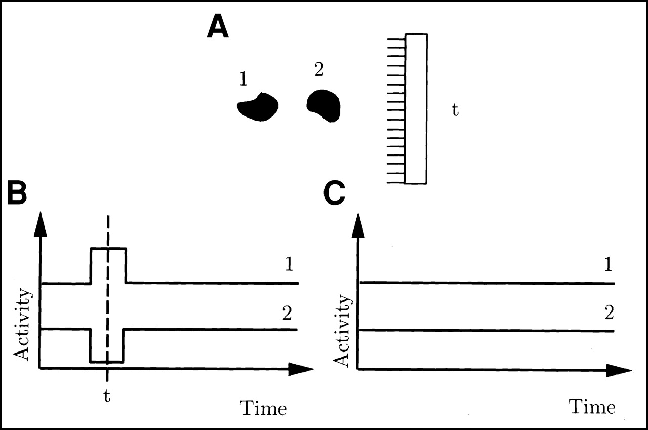
An important aspect of the reconstruction from projections is the ambiguity that occurs when the reconstruction is performed using data obtained from only 1 detector. This ambiguity leads to errors in the extracted curves. The explanation of the ambiguity is presented in Figure 7. For some projections, objects appear to overlap spatially when viewed from the direction of these projections. This allows their activity curves to be mixed during the time at which the ambiguous projection is taken without causing any change in the value of the objective function. The artifacts created by this effect can be seen in Figures 1A and 1B. The decrease in the kidney curve corresponding to the projections taken at approximately the 350th second is compensated for by an increase in the background curve at approximately the same time. This ambiguity is not present when data from >1 detector are used for the reconstruction, because at each projection different sections of the object (Fig. 7) are spatially separated on at least 1 detector. This ambiguity will not be important when other constraints are used, such as in (8), where the constraint is used so that the activity in a pixel can only increase or decrease constantly over time.

Example of ambiguity of reconstruction from 1-detector system. (A) Two objects (1 and 2) and detector head taking projection at time t. Objects overlap in this projection. Time–activity curves of these objects (B) result in set of projections identical to those that correspond to time–activity curves in C. Thus, reconstruction from such projections is ambiguous.
Another artifact can be seen in Figure 6C, where the factor coefficient image corresponding to the kidney pelvic region seems to have a star-like shape. This artifact is created because the factor for the pelvis is nonzero for only a few projections (Fig. 6C), so the image is reconstructed from only those nonzero projections. These artifacts are similar to those present in tomographic image reconstruction when there is not enough angular sampling. These streak artifacts indicate the directions at which the detectors were present at the time the factor had a nonzero value. These artifacts can be reduced using 3 detectors. Artifacts of this kind are not present in other factors that are nonzero during the entire scan (Figs. 6A, 6B, and 6D).
The reconstruction method performed well when the real canine data were analyzed. However, the observed uptake of 99mTc-MAG3 in the canine study was quite different and simpler than that in the human study. In the canine study, the kidneys appeared to have the same dynamic uptake throughout the entire volume. Therefore, the whole kidney could be treated as a single factor. In the human study, the time course for the activity was different in the kidney cortex than that in the kidney pelvis. As a result, the dynamic uptake of 99mTc-MAG3 in the kidney had to be described by 2 factors. We attribute the difference between the dynamic behavior in canine and human kidneys to different states of hydration and anesthesia of the dog and the patient. Also, in the case of the dog, the limited resolution and smaller size of the kidneys may make it difficult to see any additional components.
During the reconstruction process there was no correction performed for the detector response. As a result, there was spatial overlap between the reconstructed coefficient images (Fig. 6) that were close to each other (pelvis and cortex). This overlap prevented an easy extraction of the time–activity curves that corresponded to the kidney pelvis and the kidney cortex when both components were present in the image. There are several ways to overcome this limitation that must be considered in future work. First, correction for the detector response can be used to help improve the reconstruction, but we believe that such correction will not solve the problem completely. Second, the true physiologic curves can also be extracted directly from the projections as in (6), although the nonuniqueness problem must be addressed correctly in this approach. Third, extraction of time–activity curves from the images reconstructed by the method presented in this article can also be improved using FADS (21–23,28) instead of ROI measurements.
CONCLUSION
In this study we developed a dynamic tomographic reconstruction technique that is based on a factor model of physiologic data that allows reconstruction of the dynamic sequence of images from the data obtained from slow rotations of the camera. The efficacy of using this technique in renal studies was investigated.
The most significant motivation behind this work is that in tomographic studies proper attenuation correction can be applied, whereas in planar studies it cannot. In computer simulations we showed that we were able to accurately reconstruct the dynamics of the tracer in the kidney, even with the presence of realistic noise, when at least 2 detectors were used. Data obtained from 1 detector were not enough to reconstruct kidney dynamics without artifacts. The method extracted kidney time–activity curves in a 99mTc-MAG3 canine study and time–activity curves of the kidney cortex in a patient 99mTc-MAG3 renal study. Further studies are needed to better understand the complex dynamic of 99mTc-MAG3 in canine and patient data.
Acknowledgments
The authors thank Sean Webb for editing the manuscript. Financial support was provided by National Institutes of Health grant HL 50663 and by Marconi Medical Systems Inc.
Footnotes
Received Jan. 16, 2001; revision accepted Jun. 12, 2001.
For correspondence or reprints contact: Arkadiusz Sitek, PhD, Radiology Department, Beth Israel Deaconess Medical Center, 330 Brookline Ave., Boston, MA 02215.


