


Abstract
A slit-slat collimator combines a slit along the axis of rotation with a set of axial septa, offering both magnification in the transaxial direction and complete sampling with just a circular orbit. This collimator has a sensitivity that increases for points near the aperture slit. The literature treats this collimator as having the same sensitivity as a single-pinhole collimator, ignoring the effect of the axial septa. Herein, the sensitivity and resolution of this collimator are reevaluated. Methods: Experimental and Monte Carlo methods are used to determine the sensitivity and resolution in both the transaxial and axial directions as a function of distance from the slit (h). Eight configurations are tested, varying the slit width, septal spacing, and septal height. Results: Both the experimental and the Monte Carlo sensitivities agree reasonably with an analytic form that is the geometric mean of the pinhole and parallel-beam formulas, disagreeing with previous literature. Transaxial resolution is consistent with the pinhole-resolution formula. Axial resolution is consistent with the parallel-beam resolution formula. Conclusion: The sensitivity of this collimator is proportional to h−1 and has resolution in the transaxial direction that is consistent with pinhole resolution and in the axial direction that is consistent with parallel-beam resolution.
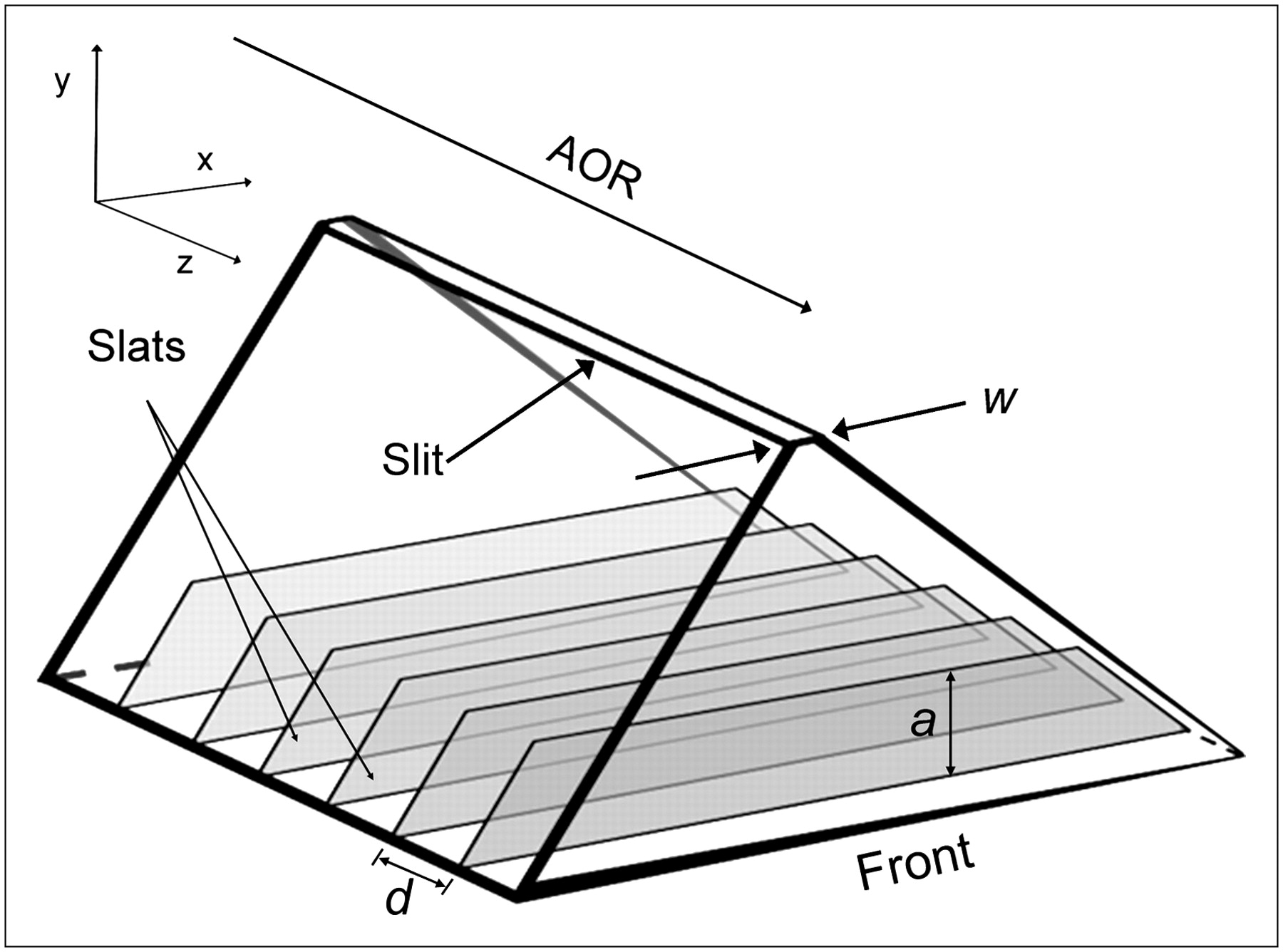
A recently published article by Walrand et al. (1) has investigated the properties of collimation that combines a slit in one direction with a set of septa spaced evenly along the direction of the slit. We also have recently begun to study this collimator, herein termed slit-slat, for possible use in human imaging. Whereas pinhole SPECT does not yield complete projection data for a circular orbit (i.e., there is not sufficient information to unambiguously reconstruct without artifacts), the slit-slat collimator (Fig. 1) does yield complete information because each axial slice of a rotating detector—with the slit parallel to the axis of rotation—yields complete information for the corresponding slice in the object. That is, each slice meets the 2-dimensional complete-sampling criteria. Other collimators with this property include parallel-beam and fan-beam. Further advantages of this collimator include fine transaxial resolution due to magnification and high sensitivity for points near the slit, as in pinhole collimation, and an enlarged axial field of view, as in fan-beam collimation. The disadvantage, compared with pinhole, is a loss of axial resolution because there is no axial magnification.

Perspective conceptual drawing of slit-slat collimator. Slit, which is parallel to axis of rotation (AOR), provides transaxial collimation. Normals to slats are also parallel to AOR. Slat height, a; slat spacing, d; and slit width, w, are indicated. x-, y-, and z-axes represent transaxial, radial, and axial directions, respectively.
The dependence of sensitivity and resolution on the parameters of the collimator is important for determining the scenarios in which slit-slat may be better than other collimation choices. Although explicit forms for the theoretic system resolution (Ro) and sensitivity (g) are not given in the article by Walrand et al. (1), both are plotted in Figure 7 therein. A careful visual inspection shows that these plots are consistent with Anger's on-axis formulas for pinhole collimation (2): Eq. 1where Ro is the overall system resolution, Rg is the geometric (collimator) component, and Ri is the intrinsic detector resolution. In addition, w is the diameter of the pinhole (edge length for a square hole), f is the focal length of the collimator, and h is the distance from the aperture plane. Moreover, these formulas do not depend on any parameters of the axial slats (e.g., height, spacing, thickness).
An alternative approach is to model a slit-slat collimator as a pinhole collimator in the transverse dimension combined with a parallel-beam (or, equivalently, fan-beam) collimator in the axial direction (parallel-beam and fan-beam are identical in the axial dimension). In that case, one would expect that Ro(pinhole) from Equation 1 would be accurate in the dimension collimated by the slit (i.e., transaxial, which is x in Fig. 1). Further, one would also expect that the parallel-beam resolution formula of Jaszczak et al. (3) would apply in the dimension normal to the slats (i.e., axial): Eq. 2where d is the gap between the septa and a is their height. (Note that the sum of the symbols a and c in Jaszczak et al. (3) equals f in Equation 2 and that b in Jaszczak et al. (3) equals h.)
It is difficult to determine from the above argument the form of the sensitivity, but an educated guess may be the geometric mean of pinhole and parallel-beam (3): Eq. 3where square holes (i.e., k = 1) have been used to match the experimental geometry, and the parallel-beam sensitivity for septa of thickness t is given by the following (3):
 Eq. 4
Eq. 4
The differences between these expectations and those of Walrand et al. (1) are pursued herein through experimental and Monte Carlo techniques.
MATERIALS AND METHODS
We use experimental and Monte Carlo methods to determine the on-axis sensitivity and resolution of slit-slat collimation.
Experimental
Setup.
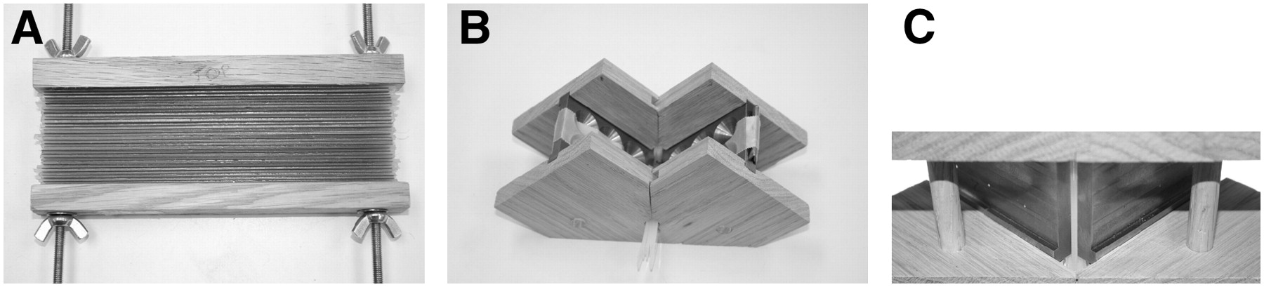
The configurations listed in Table 1 were assembled using tungsten slats (0.11 mm thick; 17 mm tall) separated by nylon spacers of thickness d (Fig. 2A); for each configuration, t = 0.11 mm. For the even-numbered configurations of Table 1, a second stack was placed on top of the first to form 34-mm-tall slats. These slats were placed on top of a large opening (39 × 61 mm) of a preexisting multiple-pinhole mount, which provided shielding from environmental photons. The slats were aligned with the transverse direction of the γ-camera (Picker Prism 3000XP; Philips Medical Systems).
Collimator Configurations

(A) Close-up of slats (17 mm tall; 0.11 mm thick), which were separated by 1.27-mm-thick nylon. (B) Close-up of slit assembly, which was formed from two tungsten plates configured to form 90° acceptance angle and separated by either 2.03 mm (shown) or 4.06 mm. (C) View of slit assembly from beneath slit.
To use preexisting material, we formed the slit from 2 tungsten plates separated by nylon spacers, obtaining a 90° acceptance angle as shown in Figures 2B and 2C. The gap between the plates (w in Eq. 1) is listed in Table 1. The slit ran parallel to the axial direction.
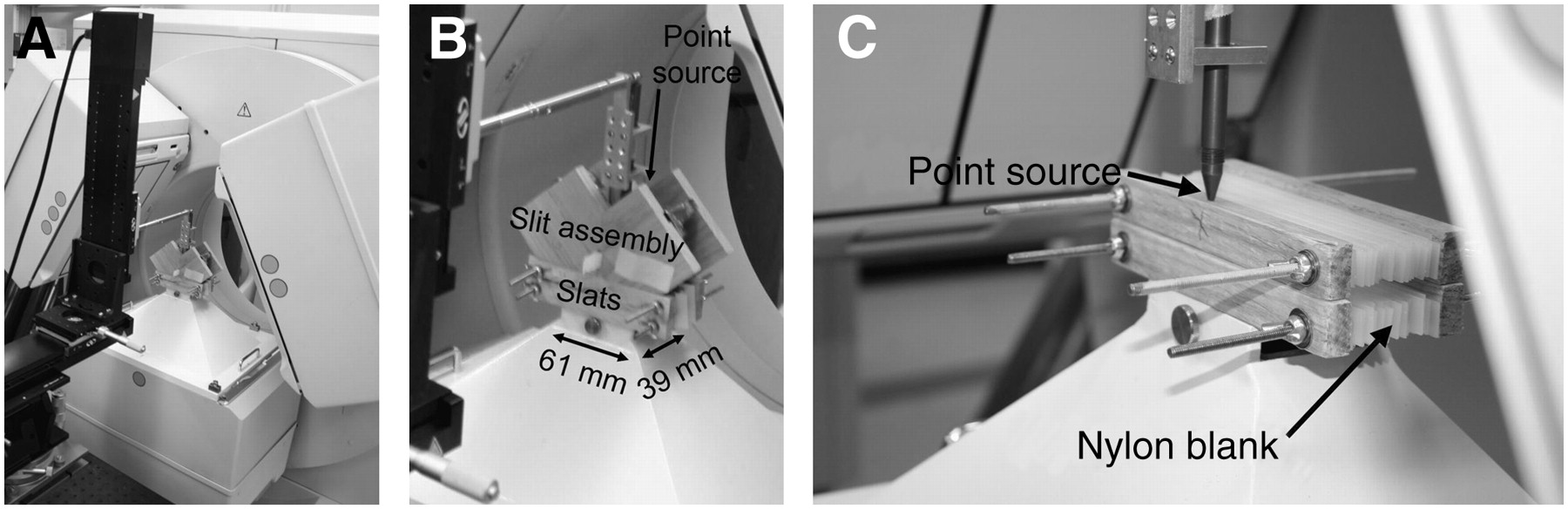
A point source (57Co; 1.3 MBq [35 μCi]) in a “pen” marker was mounted on a vertical positioning stage (Figs. 3A and 3B). The height above the slit was determined by lowering the pen until it came into contact with the support for the slats (Fig. 3C); the point source was 4 mm above the tip of the pen. The distance from the plane of the slit to the support was measured with calipers. The source was then axially centered over the hole in the shielding.

(A) Robotic stage was used to position point source above aperture slit (h = 10−205 mm). (B) Zoom of (A) with labeled slit assembly and slats; 39 × 61 mm opening in shielding is also indicated. (C) Source was brought into contact with support of “blank” slats as reference point in determining h.
Data Acquisition.
Projections of the 57Co point source were acquired for 60 s each at distances of 10–205 mm above the aperture plane in increments of 5 mm for each of the configurations listed in Table 1. The energy window was set at 15%. The projections were 256 × 256 bins (1.11-mm edge length). These data were used for sensitivity and transaxial resolution measurements.
To smooth the axial profiles for a resolution measurement, a robotic stage moved the septa linearly in the axial direction over one period (d + t) during each view to average over one period of the slat-spacer pattern. This dedicated experimental run was used only for the measurement of axial resolution. Other acquisition parameters were identical to those described in the previous paragraph.
An additional “blank” dataset was taken with a blank-septa assembly and without the aperture slit (Fig. 3C). The blanks were made of nylon and were similar to the tungsten-slat configuration except that the tungsten slats were removed. This dataset was used to determine normalization for sensitivity and focal length. Further, a dataset was acquired without the point source present to assess the background.
Sensitivity Normalization.
The blank dataset was analyzed to determine the effective product of the source emission rate and the camera efficiency. The central 46 bins in each dimension (2,116 bins in total), covering an area of about 2,619 mm2, were chosen as a region of interest. The counts in this region were fit as a function of h to the equation: Eq. 5where A is the area of the region of interest (2,619 mm2), C is the emission counting rate of the source per acquisition frame, ε is the overall system efficiency, and f is the distance from the aperture plane to the detector (i.e., the focal length). Thus, this equation is the flux of photons on area A times the efficiency of detection. This equation was fit for the product Cε and for f. Background was estimated by averaging the scan without a point source present and a region of interest at each h that was far from the projection through the slit. The number of counts in each experiment less background and corrected for attenuation in the nylon spacers (19% (4)) was then divided by this Cε to determine sensitivity. This sensitivity is equivalent to that for an idealized collimator that does not have attenuating spacers.
Resolution Measurement.
For each experimental configuration at each value of h, the axial slices of a region of interest of the projection were summed to form a transverse profile, and the transaxial slices of that region were summed to form an axial profile. These profiles were corrected by subtracting a flat background, which was measured with the background scan. The maximum of each adjusted profile was determined. The full width at half maximum (FWHM) was then calculated by interpolating the location of the half maximums. The transverse resolutions were scaled to object space by dividing by the magnification f/h. Axial resolutions were not scaled, because axial magnification is unity.
Monte Carlo
A Monte Carlo simulation was performed to model the slit-slat collimator. The model consisted of an infinite slit along the z direction and axial slats normal to this direction (Fig. 1). Each run modeled 5 × 10⁸ photons emitted isotopically from a point source at each position h; the values of h ranged from 10 to 205 mm in steps of 5 mm. In one mode of the simulation, the collimator material was considered to be infinitely attenuating so that only photons that did not intersect any material in the slit or septa were counted; another mode allowed both slit penetration (linear attenuation coefficient of 4.95 mm−1 (4)) and detector parallax (5) (linear capture coefficient of 0.374 mm−1 (4)). Eight configurations were used (Table 1). For each configuration, t = 0.11 mm. Further, each configuration was run with and without modeling the hole at the top of the lead box that was used for mounting the septa (Fig. 3B); this lead box limited the axial field of view.
The purpose of the Monte Carlo that models the hole at the top of the lead box is for comparison with experimental data that are particular to the setup described herein. The purpose of the Monte Carlo without this modeling is for comparison with the more idealized theoretic form of Equation 3.
RESULTS
The experimental and Monte Carlo results for sensitivity are shown in Figure 4, with Equations 1 and 3 for g(pinhole; k = 1) and g(pinhole|parallel-beam), respectively. The experimental sensitivity was computed by dividing the net number of experimental counts in a 60-s frame by the product Cε, which was measured to be 37.2 × 10⁶ counts (0.620 MBq × 60 s) by fitting Equation 5 to the blank-scan data. Two cases are shown for the Monte Carlo data. In one case, labeled in Figure 4 as “MC,” only photons passing through the opening at the top of the shielding were counted; this better matches the experimental conditions. In the other, labeled in Figure 4 as “MC no truncation,” the photons were not constrained to pass through the opening, matching the expectations of the slit-slat concept: a long slit complemented with axial septa. Both cases allow penetration of the tungsten aperture slit and slats. Although not shown in Figure 4, Monte Carlo without penetration and not constrained to be within the shielding opening is consistent with Equation 3.
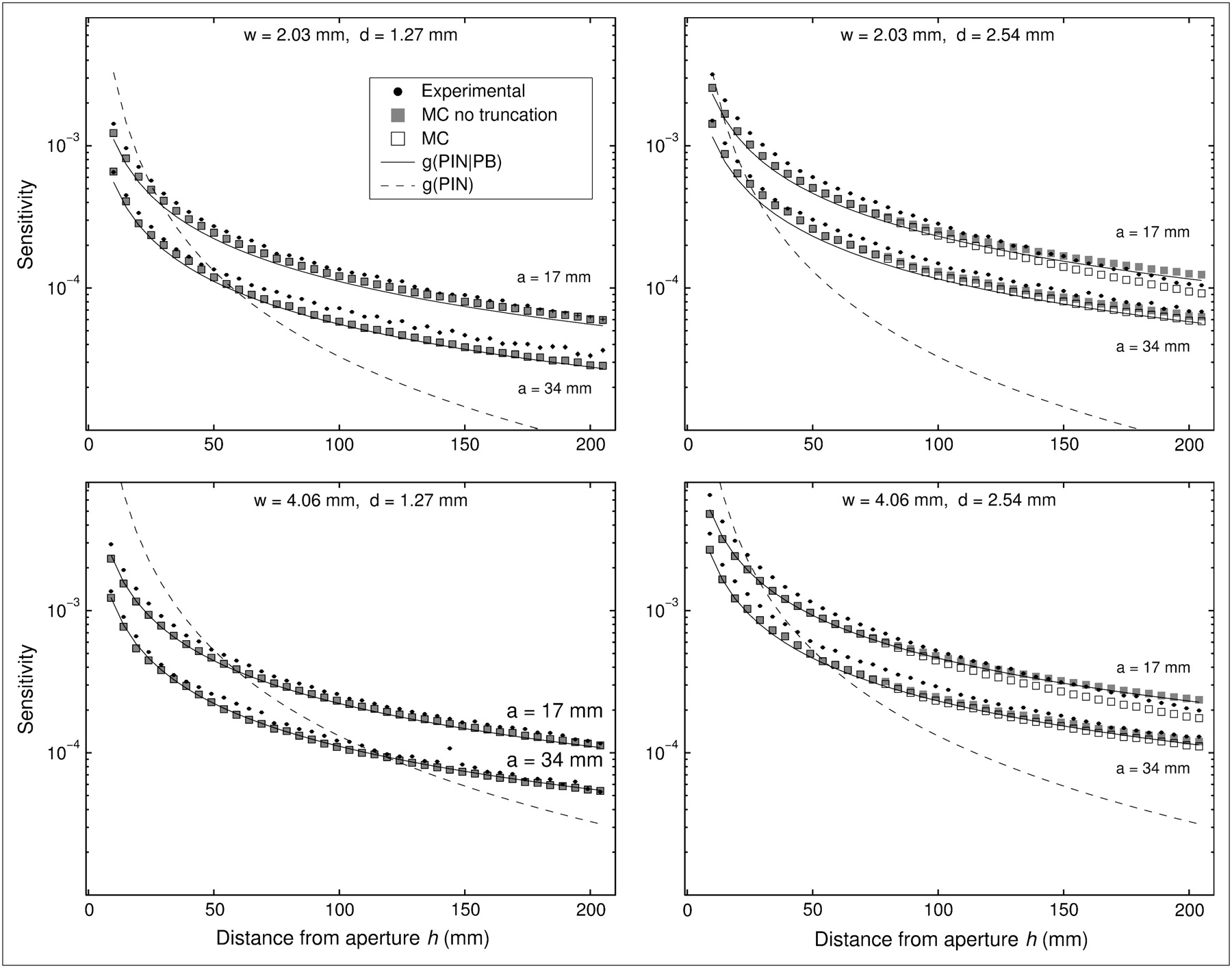
Sensitivity of slit-slat collimation. Experimental and Monte Carlo results (both with and without modeling of truncation from opening in shielding) are shown with g(pinhole|parallel-beam) and g(pinhole; k = 1). The results are shown for w = 2.03 mm (top) and w = 4.06 mm (bottom) and also for d = 1.27 mm (left) and d = 2.54 mm (right). Within each plot, a = 17 mm appears on top and a = 34 mm appears on bottom. PB = parallel-beam; PIN = pinhole.
The experimental and Monte Carlo results for transaxial resolution are shown in Figure 5. These resolutions have been scaled to object space by multiplying the FWHM resolution on the detector by h/f. The statistical uncertainty was estimated through bootstrap resampling of the profiles (6). The Monte Carlo results show two cases. The case labeled “MC full” includes the effects of slit penetration and detector parallax on the resolution. The case labeled “MC simple” does not include these effects. The theoretic prediction of Equation 1 for Ro(pinhole) is also shown.

Transaxial resolution (FWHM) of slit-slat collimation. Experimental and Monte Carlo results (both with [full] and without [simple] modeling of penetration and parallax) are shown with Ro(pinhole). Results are shown for d = 1.27 mm (top) and d = 2.54 (bottom) and also for a = 17 mm (left) and a = 34 mm (right). Within each plot, w = 2.03 mm appears on bottom and w = 4.06 mm appears on top. PIN = pinhole.
Figure 6 shows the experimental results for axial resolution. These resolutions are the same on the detector and object planes. The statistical uncertainty was estimated through bootstrap resampling of the profiles (6). The Monte Carlo results show two cases. The Monte Carlo labeled “MC” is constrained to be within the shielding opening (i.e., it models truncation). “MC no truncation” does not include this effect. In addition, the theoretic prediction of Equation two for Ro(parallel-beam) is also shown.
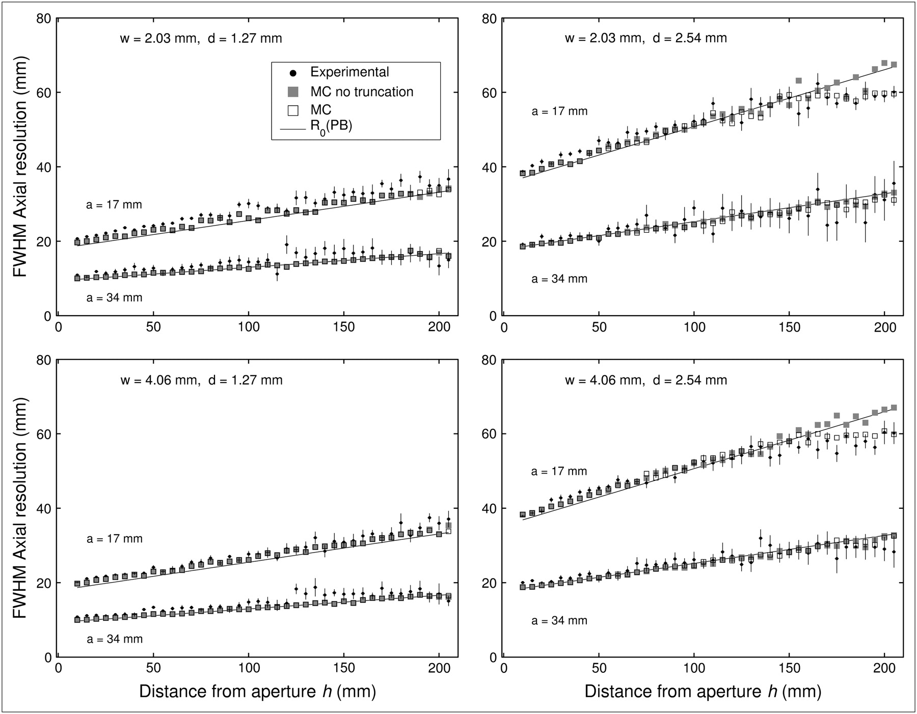
Axial resolution (FWHM) of slit-slat collimation. Experimental and Monte Carlo results (both with [full] and without [simple] modeling of axial truncation) are shown with Ro(parallel-beam). Results are shown for w = 2.03 mm (top) and w = 4.06 mm (bottom) and also for d = 1.27 mm (left) and d = 2.54 mm (right). Within each plot, a = 17 mm appears on top and a = 34 mm appears on bottom. PB = parallel-beam.
DISCUSSION
Overall, the sensitivities for the 8 configurations shown in Figure 4 agree with Equation 3 over a large range of h and for values of w, d, and a varying by factors of 2. The Monte Carlo results also show consistency with the experimental data and Equation 3. On the other hand, the experimental and Monte Carlo results are inconsistent with the form of g(pinhole) from Equation 1.
Equation 3 by itself does not take into account the effect of slit penetration. The Monte Carlo results allow for this penetration, which increases sensitivity. When the Monte Carlo does not allow penetration, it agrees numerically very well with Equation 3 (results are not shown for brevity). Perhaps the effects of penetration can be well modeled by an effective diameter (2,7). By comparing Monte Carlo with and without penetration, one finds for 57Co and tungsten that weff = 2.20 for w = 2.03 mm and weff = 4.20 for w = 4.06 mm. Thus, penetration was found to be a relatively small component in this experiment. Monte Carlo data fall between the experimental and theoretic results, suggesting that penetration accounts for some of the difference between theory and experiment. Scatter, which is not included in the Monte Carlo or Equation 3, is likely to account for at least some of the remaining difference.
For Figures 4B and 4D, where d = 2.54 mm, the trend of the experimental data for a = 17 mm does not track the trend of the Monte Carlo without truncation for values of h greater than about 100 mm. However, the trend matches that of the Monte Carlo with truncation, which counts only photons that pass within the hole at the top of the shielding. Thus, in these cases, the axial resolution is so large that some of the photons are truncated; indeed, axial resolution is expected to be larger for both larger d and smaller a (Eq. 2). Overall, Equation 3 provides accurate predictions for the sensitivity within a small factor.
Figure 5 shows that Ro(pinhole) of Equation 1 yields a reasonable prediction for both the experimental and the Monte Carlo transverse-resolution data. For small values of h, Equation 1 and the “simple” Monte Carlo tend to underestimate the experimental resolution because they do not include the effects of slit penetration and detector parallax, which have their greatest effects on resolution at small h; the “full” Monte Carlo includes these effects and agrees well with the data even at small h.
Figure 6 shows that Ro(parallel-beam) of Equation 2 yields a prediction that is consistent with both the experimental and the Monte Carlo data. However, the resolutions are inconsistent with the predictions of pinhole resolution, which are not shown. For comparison with the data in Figure 6, Ro(pinhole) would need to be scaled by f/h because the results were calculated on the detector plane and Ro(pinhole) was calculated on the object plane. When scaled, the prediction would decrease with h because the projection size of a point decreases with h. In contrast, Figure 6 shows that the resolution on the detector plane increases (degrades) with h. Further, whereas the data clearly increase with increasing d and decreasing a, the pinhole prediction does not.
For Figures 6B and 6D, when a = 17 mm there is a deviation from the prediction of Equation 2 when h is large. Monte Carlo data not modeling truncation continue to agree with Equation 2, whereas Monte Carlo data modeling truncation follow the data. Thus, in the experimental configuration used, large values of h led to truncation that interfered with resolution measurements. Overall, the data suggest that Equation 2 is a good model for axial resolution.
In the configuration used for the experiment, we found that measuring axial resolution with a FWHM metric posed difficulties due to the appearance of shadows from the slats in the projection. These shadows resulted from relatively short septa (i.e., a was small) and from their being positioned near the slit rather than near the detector. The projections had several local minima, making the numeric determination of FWHM complicated. Consequently, a dedicated experiment was performed to measure axial resolution by “wobbling” the axial slats. That is, the slats were linearly moved in the axial direction by one period (d + t) during each projection view. This movement had the effect of averaging out the shadowing, resulting in the expected triangular shape of the profiles.
Limitations in the experimental apparatus caused truncation for large values of h when the axial resolution was large (d = 2.54 mm; a = 17 mm). Materials used to set up the experimental apparatus were chosen because they were available to us in our laboratory, and the apparatus will be redesigned in future performance evaluations of clinical configurations. In future experiments involving an actual collimator, nylon will be removed or replaced by a less attenuating material. However, the use of nylon spacers was a convenient and readily available method for keeping the slats evenly spaced and straight.
Walrand et al. (1) suggested theoretic values for resolution and sensitivity of this slit-slat collimator. The data herein show that those predictions were inaccurate for sensitivity. The predictions for transaxial resolution were accurate (Ro(pinhole) in Fig. 5) but can be improved by modeling slit penetration and detector parallax. It is unclear if Walrand et al. (1) intend for the pinhole resolution formula (Eq. 1) to be applied in the axial direction as well as in the transverse direction. The data make clear that application in the axial direction would not be accurate.
The implications of the sensitivity and resolution formulas suggest that this collimator may be less useful for small-animal imaging than is a pinhole collimator because the sensitivity does not increase as rapidly for a small radius of rotation and the axial resolution does not improve as rapidly because there is no axial magnification. On the other hand, this collimator is likely to have a niche between pinhole collimation and parallel-beam/fan-beam collimation because the sensitivity improves with decreasing distance (unlike parallel-beam and fan-beam) but does not drop as rapidly as for pinhole collimation as distance increases. Further, transaxial magnification aids transaxial resolution by mitigating the effect of intrinsic detector resolution. Lastly, because the collimator provides complete data with a circular orbit, there will be no artifactual axial blurring as in pinhole SPECT using a single circular orbit.
CONCLUSION
Slit-slat collimation may be well described as a hybrid of pinhole and parallel/fan-beam collimation. Its on-axis sensitivity is well described as the geometric mean of these collimators (Eq. 3). Its resolution is described well by the pinhole resolution formula (Eq. 1) in the transaxial direction. Axial resolution is consistent with the parallel-beam formula (Eq. 2). Because this collimator has a distance dependence of h−1 for its sensitivity, it falls between pinhole and parallel/fan-beam. It is likely to be useful in intermediate scenarios such as imaging of limbs, the breast, medium-sized animals, and, possibly, the brain.
Acknowledgments
This research was supported by the National Institute for Biomedical Imaging and Bioengineering of the National Institutes of Health under grants R01-EB-001910 and R33-EB-001543 and by the U.S. Army Contracting Agency under contract DATM05-02-C-0034. The authors thank Dr. Richard Lanza for use of the tungsten slats, Dr. Richard Freifelder for assistance with the experimental setup, and Joshua Scheuermann for help with graphics design.
References
- Received for publication May 9, 2006.
- Accepted for publication July 26, 2006.


