


Abstract
This article, the first in a 2-part series, provides an introduction to machine learning (ML) in a nuclear medicine context. This part addresses the history of ML and describes common algorithms, with illustrations of when they can be helpful in nuclear medicine. Part 2 focuses on current contributions of ML to our field, addresses future expectations and limitations, and provides a critical appraisal of what ML can and cannot do.
It seems that currently every conference hosts sessions on artificial intelligence (AI) and machine learning (ML) and that these terms are increasingly pervading our literature. However, AI and ML are not new. First described in 1956, the term artificial intelligence refers to computers that perform tasks normally requiring human intelligence (e.g., visual perception or decision making). ML, a branch of AI, dates to the electronic computing of the 1950s (1) and its application to medicine in the 1960s (2).
Broadly speaking, ML refers to algorithms that are programmed to learn from observations and can then make statistical inferences based on what has been learned, rather than being based on the explicit knowledge of the programmer. Traditionally, a programmer specifies all aspects of an algorithm and nothing further is learned beyond what has been written, like writing a detailed recipe for baking a cake. ML algorithms include parameters with unknown values at the time of programming that are learned by presenting the program with observations, like a novice chef using an incomplete recipe to bake a cake. The chef must decide what ingredients to use and in what proportion, based on observations.
Why the rise in ML algorithms for medical imaging now? Reasons include advances in theory (better algorithms) (3), microelectronics (better hardware) (4), and availability of massive amounts of training data (i.e., big data). Also, fields such as radiomics and radiogenomics have shown great promise (5). Radiomics refers to the extraction and quantification of mathematic descriptors (known as features) of image texture, shape, and other qualities, which can be correlated with a variety of data, such as histopathologic findings and clinical outcomes (survival). Radiogenomics more specifically correlates radiomic features with genomic data. These new fields use ML to investigate scientific phenomena by identifying often previously unknown relationships.
The aim of this article, the first in a 2-part series on ML in nuclear medicine, is to introduce ML and discuss common algorithms, highlighting differences between them. The second article will address future expectations and limitations and provide a critical appraisal of what ML can and cannot do.
A BIRD’S-EYE VIEW OF ML ALGORITHMS
ML algorithms include core elements: a mathematic model, a cost function, and data. The art is identifying the mathematic model and cost function suitable to the task and finding access to sufficient data.
Mathematic Model
A mathematic model is a way to explain relationships between data and to translate input observations into outputs. For example, a mathematic model could be a function that translates input features from an image (e.g., the SUV ratio [SUVR] for amyloid brain PET in a region of interest [ROI]) into an output decision (e.g., scan classification as positive or negative for amyloid deposition). The decision of which model to use is often based on tradeoffs between accuracy, suitability for the task, and practical implementation considerations. Problems for which the model’s output observation is continuous-valued (e.g., amount of amyloid deposited) are known as regression problems; those with discrete-valued output observations or categories (e.g., amyloid-positive or -negative) are known as classification problems. Mathematic models vary and have different levels of complexity or predictive capability. Many models have parameters called hyperparameters, which are chosen before training but may be adjusted if performance is insufficient. For example, it might be initially stipulated that any given amyloid brain PET result is classified as positive or negative for amyloid deposition (e.g., 2 outcomes allowed); however, training could suggest that some scans are equivocal (e.g., 3 outcomes allowed).
Cost Function
A cost function (or loss function) measures how close the model performance is to its intended result. For example, the cost function could be a misclassification rate or mean square error.
Data
Just as physicians learn by reviewing cases, an ML algorithm is trained using data. Data may be image measurements (e.g., SUVRs for an amyloid PET study), survival data, or a combination of these and other observations. Data are usually divided into training, validation, and testing subsets. Training data are used to teach the model, validation data are used to fine-tune hyperparameters, and testing data are used to confirm the performance of the trained model. Often, the data include known outputs. For example, a physician might have classified all available amyloid PET scans as amyloid-positive or -negative. Sometimes, outputs are unknown. For example, one might have all the SUVRs for the ROIs but not know if the scan is amyloid-positive or -negative. Whether the data include known outputs distinguishes 2 broad ML algorithm categories: supervised and unsupervised.
SUPERVISED AND UNSUPERVISED LEARNING
Supervised learning refers to ML algorithms that are trained using known outputs. For example, an ML algorithm could determine neurologic outcomes using knowledge of prior SUVR/ROI combinations and neurologic findings. In a sense, supervised algorithms determine unknown parameters of a mathematic model based on the training data in view of predicting outcomes for future test data. Examples of supervised ML algorithms, described below, are linear regression, support vector machines, random forests, and artificial neural networks (ANNs).
Unsupervised learning refers to ML algorithms that use training data for which outputs are unknown. These algorithms often solve tasks such as identifying commonalities between data points (e.g., clustering amyloid PET into amyloid-positive or -negative with no a priori knowledge of which category the PET scan belongs to) or finding ways to compress data (e.g., reducing the number of features required to predict an outcome). Examples of unsupervised ML algorithms, described below, are k-means clustering, principal component analysis, and singular value decomposition.
There are also ML algorithms that are not strictly supervised or unsupervised (e.g., reinforcement learning, competitive learning, and semisupervised learning). These are beyond the scope of this paper.
Figure 1 illustrates these concepts theoretically. In Figures 1A and 1B, the data points are classified into circles and triangles. In Figure 1C, the data points are not classified. If the purpose is to train an ML algorithm to appropriately classify data into circles and triangles, and the classification scheme is known, a supervised approach is preferred. For a scenario in which the classification scheme is unknown, assigning data to categories requires an unsupervised approach. An observer might say there are 2 clusters of data points (bottom left and top right). However, another observer might group data points into more clusters. Ultimately, an initial educated guess on the number of categories might be necessary. Figures 1D–1F show potential models applied to each scenario. In Figure 1D, a straight line creates a delineation between circles and triangles. The mathematic model in this case is linear, namely y = ax + b, and the ML algorithm must learn the values of a and b that minimize the number of false classifications (e.g., minimizes the cost function). In Figure 1D, line 2 has a lower cost than line 1 because the number of triangles in the region of circles is less. An effective ML algorithm could adapt a and b toward the better solution. In Figure 1E, a linear model would inevitably lead to a high number of false classifications. In this case, a more complex nonlinear model might be better suited for this task. In Figure 1F, an algorithm categorized data into 2 clusters. Several common ML algorithms are discussed below and summarized in Table 1.
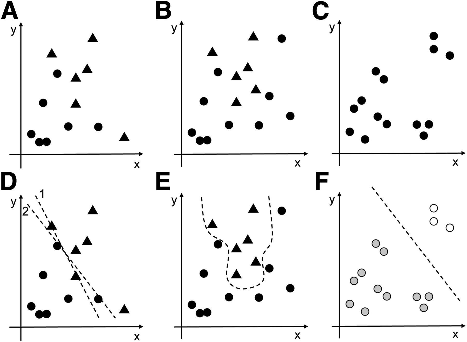
ML tasks. (A and B) Input measurements classified as circles or triangles for supervised learning (e.g., triangles could be positive cases, and circles negative cases). (C) Input measurements not classified (e.g., clinical information unknown). (D) A better fit for classification using line 2 than line 1. (E) Classification requiring nonlinear approach. (F) Potential clustering.
Key Aspects of ML Algorithms
COMMON ML ALGORITHMS
There are many ML algorithms, typically programmed in languages such as R, Matlab, and Python (6) that include built-in support (e.g., as libraries, toolkits, or packages). Many aspects differentiate these algorithms, and the best algorithm to use often depends on the task, data, and mathematic model complexity (e.g., number of operations such as additions and multiplications to be performed).
Naïve Bayes Classification
The naïve Bayes classification is a supervised algorithm that classifies features that follow a simple probability distribution (e.g., Gaussian or multinomial) and assumes that the features are independent of each other (allowing mathematic simplifications). The hyperparameters are the distribution parameters (e.g., mean and variance of feature values for each class). Classification is done by looking at features and computing the class that maximizes a probability function. The computational cost is low. For example, a retrospective study by Mehta et al. used a multinomial naïve Bayes classifier to predict response to 90Y radioembolization therapy from 18F-FDG PET/CT features (7). Using 22 training cases and 8 testing cases, the sensitivity for predicting response was approximately 80%.
Linear Regression
Linear regression is a supervised algorithm for regression problems in which datasets contain n-dimensional continuous features, and the model is the n-dimensional hyperplane (hence the linearity) that best fits the dataset. The cost function is defined as the mean square error between the true outcomes and the model’s predicted outcome. The computational cost is low.
Support Vector Machines (Fig. 2)
A support vector machine is a supervised algorithm for binary classification or, less commonly, regression. The algorithm identifies a curve (or hypersurface, if there are many dimensions) that best separates 2 classes in such a way that the curve is at maximum distance from the closest points in each class. The closest data points to the line are called the support vectors, hence the algorithm name. Once trained, support vector machines tend to be computationally efficient, at least for smaller datasets (e.g., once trained, the algorithm need only determine which side of the curve a new data point is on). Support vector machines can also handle data for which no clear linear separation (hyperplane) can be drawn between classes (Fig. 1B), by moving to a higher-dimension space, using a nonlinear data transformation, or minimizing the number of misclassifications. For example, Van Weehaeghe et al. used a support vector machine to classify subjects as amyotrophic lateral sclerosis (ALS) patients versus healthy controls based on differences in brain metabolism on 18F-FDG PET (8). All PET data were spatially normalized and analyzed quantitatively using a volume of interest and voxel-based analysis with statistical parametric mapping protocols. A cohort of 70 ALS and 20 healthy subjects trained a support vector machine (linear model) using a voxel-based comparison and a brain mask defined by those voxels exceeding 50% of the mean of the 18F-FDG PET images. Subsequently, 105 ALS subjects served as test data showing the support vector machine was 100% accurate for classification. Since ALS subjects had similar patterns of brain metabolism in both the training and the testing data, the support vector machine was able to correctly distinguish subjects with ALS from healthy controls. There would have been little need to explore a more computationally intensive ML algorithm to solve this task. Of interest, 10 subjects with primary lateral sclerosis were also recruited. Since brain metabolism in ALS and primary lateral sclerosis was similar, these subjects could not be discriminated and further evaluation would be needed to classify these cases.

Illustration of support vector machine. (A) Training dataset shown as scatterplot. (B) Solid line with maximum distance to closest data points in each category; solid points indicate closest points, known as support vectors. There are no data points in region between dashed lines.
Random Forest (Fig. 3)
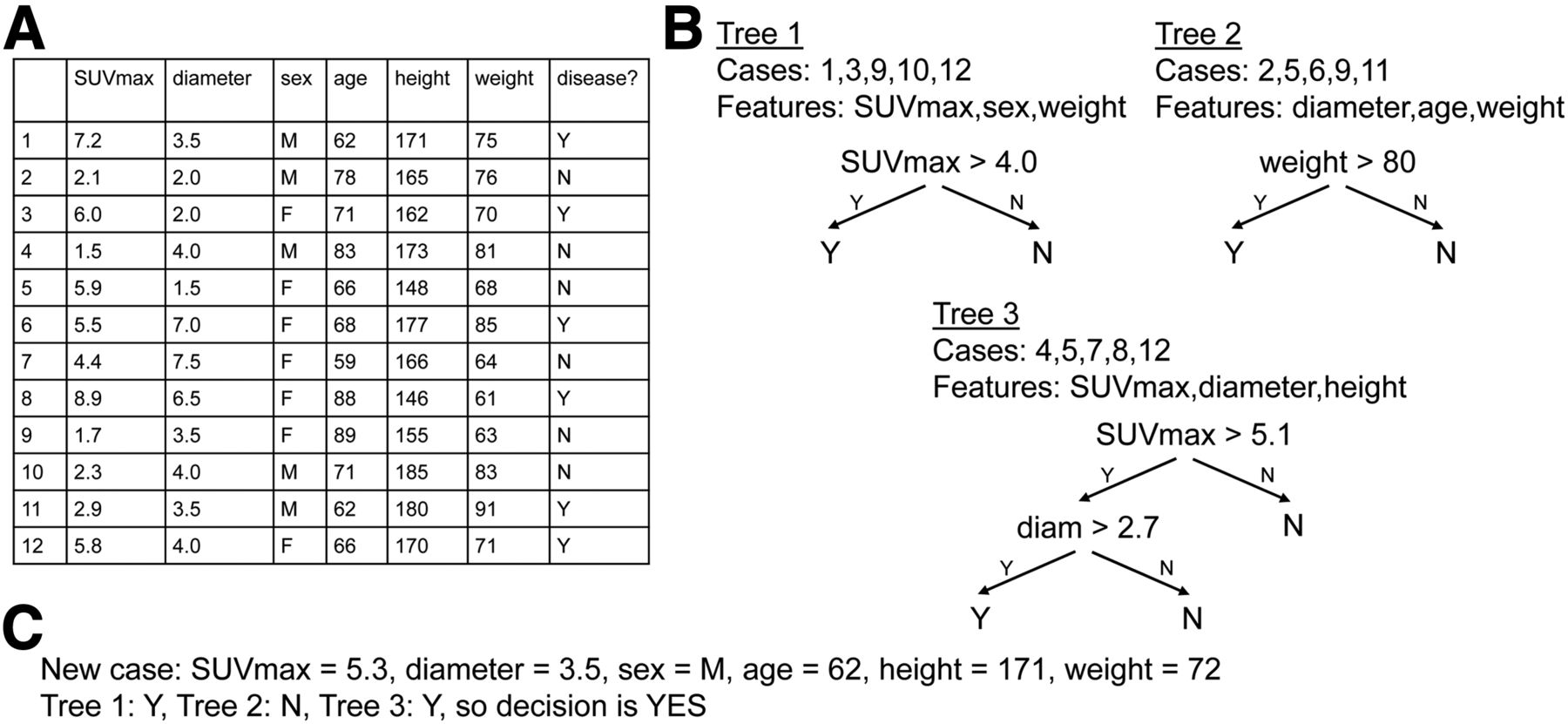
A random forest is a supervised algorithm that creates a collection of decision trees (i.e., forest) for classification or regression. For example, one might want to predict neurologic findings by learning from a series of SUVR/ROIs on amyloid PET scans in patients with known neurologic findings. To build each tree in the forest, the algorithm picks a random subset of cases and a random subset of features (the sizes of these subsets are hyperparameters). In our example, the subset of cases is randomly chosen from the amyloid PET scans with clinical reads, and the subset of features is randomly chosen from the available ROIs. Each tree is recursively constructed starting at the root by identifying the feature (e.g., ROI) and feature value (e.g., SUVR) that best (according to misclassification rate) splits the subset’s cases into a left pile and a right pile; then, 2 branches are created in similar fashion: a left branch for the left pile and a right branch for the right pile. The endpoints of the trees represent the outputs and are reached when a pile has cases from only 1 class (e.g., all negative or all positive); the endpoints can be classes (for classification problems) but may also be numeric (for regression problems). Each tree is different since it deals with different subsets of data. Once the forest has been created, new data are presented to each tree for categorization; the final result is the most common decision among all trees’ decisions. In our example, the final result could be the clinical finding (class) that is most common: positive or negative for amyloid deposition. As a recent study showed, a random forest with 2,000 trees could be trained to predict subject mortality after 90Y radioembolization in a group of 366 subjects with intrahepatic tumors based on factors such as age at radioembolization, liver function, and tumor burden (9). Here, the authors used a parameter, minimal depth (i.e., shortest distance in a tree from trunk to branch of first split in the variable), to identify predictive measurements: baseline cholinesterase and bilirubin. In particular, postprocedural mortality was found to increase significantly once bilirubin levels exceeded 1.5 mg/dL.

Illustration of random forest. (A) Training dataset with 12 cases, each with 6 features, and outcome for supervised training. (B) Three trees, each generated from 5 randomly selected cases and 3 randomly selected features; for trees 1 and 2, 1 feature is sufficient to fully separate 5 cases, and for tree 3, 2 features are needed. (C) New case in which trees 1 and 3 return Y and tree 2 returns N; therefore, majority decision is Y.
ANNs (Fig. 4)
ANNs are typically (but not always) supervised and can be used for classification or regression problems. ANNs process data in steps (called layers). At each layer, several simple computation units called neurons (inspired by biology) process input data and convey results to neurons in the next layer (Fig. 4A). A neuron’s computation typically involves a weighted summation of inputs and a bias, followed by a nonlinear transformation of the result (e.g., thresholding). An algorithm such as backpropagation (10) is used for training (e.g., learning values for weights). Among ML algorithms, ANNs tend to be the most powerful but also the most computationally challenging. The computational cost comes from the fact that normally, every neuron in a layer is connected to every neuron in the subsequent layer. To illustrate how this can become problematic, consider an ANN that processes a 100 × 100 pixel image, for example, with 10,000 inputs. If each layer has as many neurons as there are inputs, each layer requires 10,000 × 10,000 = 108 connections, each of which requires at least 1 multiplication and addition, hence the high computational cost per layer. In the earlier days of ML, ANNs were limited by this high computational cost (which could not be met by the microelectronic technologies of the time) and the fact that some problems remained unsolvable (although it could be argued they would have been solvable had the proper technology been available). Recent developments have allowed ANNs to overcome these barriers, and ANNs are now very popular.

(A) ANN with 4 layers, and neurons (circles). Arrows indicate values passed from one layer to another. (B) Sample CNN for brain PET processing. Two layers each perform 2-dimensional convolution followed by rectified linear unit (ReLU) and pooling (taking maximum value of every 4 pixels to reduce total number of pixels). Resulting matrix (feature map) is flattened into 1-dimensional array of neurons that are fully connected to another layer. Nonlinear operation (soft max) is performed to generate classification. For simplicity, we show single-input slice; however, CNNs can process higher-dimension or multimodality images. Parameters include number of layers, number of pixels in convolutional filter, convolution stride, and number of pixels pooled, called hyperparameters. (C) Image processing used by Walker et al. (23), with 2 paths processing images at different scales, each with contrast-limited adaptive-histogram equalization (CLAHE), deep CNN, and subsequent random forest.
Deep learning, first described in 1986 (11), was applied to ANNs in 2006 (12) to form deep neural networks (DNNs). DNNs are essentially ANNs with many layers (10–150, depending on the task). By having a large number of layers, DNNs are more computationally taxing but are able to tackle complex problems. Also, each DNN layer is thought to treat data at a different level of abstraction. For instance, a DNN might devote a first layer to image segmentation and a subsequent layer to lesion identification within a segmented ROI.
The high computational cost per layer can be reduced using structures whereby each neuron connects to a subset of neurons in the subsequent layer. A method for image-processing applications is a convolutional neural network (CNN). CNNs are a form of DNN in which the main difference is the use of convolutional layers. Specifically, in a CNN, the outputs of neurons at 1 layer are considered to be an image; 2-dimensional convolution is applied to the image, followed by a nonlinear operation (called ReLU, for rectified linear unit) and pooling of pixel data (combining several pixels into one, which also reduces cost). Say a convolutional mask of size 10 × 10 is used in the example above, only 10,000 × 100 = 106 multiplications and additions are required—a 100-times savings. Figure 4B depicts a 2-layer CNN in which each performs a convolution, ReLU, and pooling. After these layers, another layer of neurons (with each neuron being connected to every neuron in the previous layer) computes the output classification. Also, CNNs can be used to directly process images but can also be used with predefined ROIs or volumes of interest. Thus, there is no need to decide which radiomic features to extract, as the CNN can make its own choice of features. In 2012, a breakthrough occurred with the introduction of a CNN called AlexNet5 (13) that outperformed prior ML algorithms in an open challenge called ImageNet.
Together, DNNs and CNNs (indeed, there is little distinction between the two in the literature, and most ANNs today are both deep and convolutional, to the point where all 3 acronyms are nearly used interchangeably) paved the way for the current boom in ML. In general, deep learning requires less human input for training purposes than more traditional ML algorithms. Unfortunately, deep learning is also more complex and often requires a large amount of training data to be effective. For example, in the ImageNet challenge (13), more than 1 million annotated images were used. In medical imaging, it is often difficult to acquire such large numbers of training samples. To circumnavigate this limitation, researchers have tried to reduce requirements for training data by using data-augmentation techniques (14–16), reducing image dimensionality (16–19), and fine-tuning existing pretrained DNNs (19–21). For example, in some cases the available data can be slightly varied—such as by rotating images, flipping images, or adding noise—to augment the data. Also, if layers of a network can be trained on a set of images with similar features to the images being studied, this learning might be transferred to the new task, known as transfer learning, decreasing the data needed to learn the new task.
CNNs have been used in several medical imaging settings. In a nice example, CNNs have been used in conjunction with image preprocessing and random forests in an automated system to detect malignancy on mammograms (22). A sequence of image-processing steps optimized using genetic algorithms was applied (Fig. 4C). Mammograms were preprocessed using a technique called contrast-limited adaptive histogram equalization. This was followed by 2 deep CNNs (each with at least 20 layers) that processed images at 2 different scales, and then a random forest made a final prediction. A dataset with over 7,000 images divided into training, validation, and test sets reportedly resulted in an ML algorithm with comparable sensitivity and specificity to that of a radiologist.
Principal Component Analysis (Fig. 5)
Principal component analysis is an unsupervised algorithm for data simplification. The idea is to find linear combinations of building blocks (e.g., features) that can be used to reconstruct the initial data, with the combination of building blocks being simpler than the initial data and any initial data loss minimized. Principal component analysis is often used for data compression. An example of principal component analysis in nuclear medicine is to reduce respiration artifacts in PET scans (23). In this case, the task requires identifying the data that are most suggestive of breathing and using this information during the reconstruction process to reduce breathing artifacts. The authors showed a high correlation between principal component analysis and results obtained using costly external gating equipment. Linear discriminant analysis is closely related to principal component analysis. The fundamental difference is that linear discriminant analysis is a supervised algorithm that requires linear combinations of building blocks.

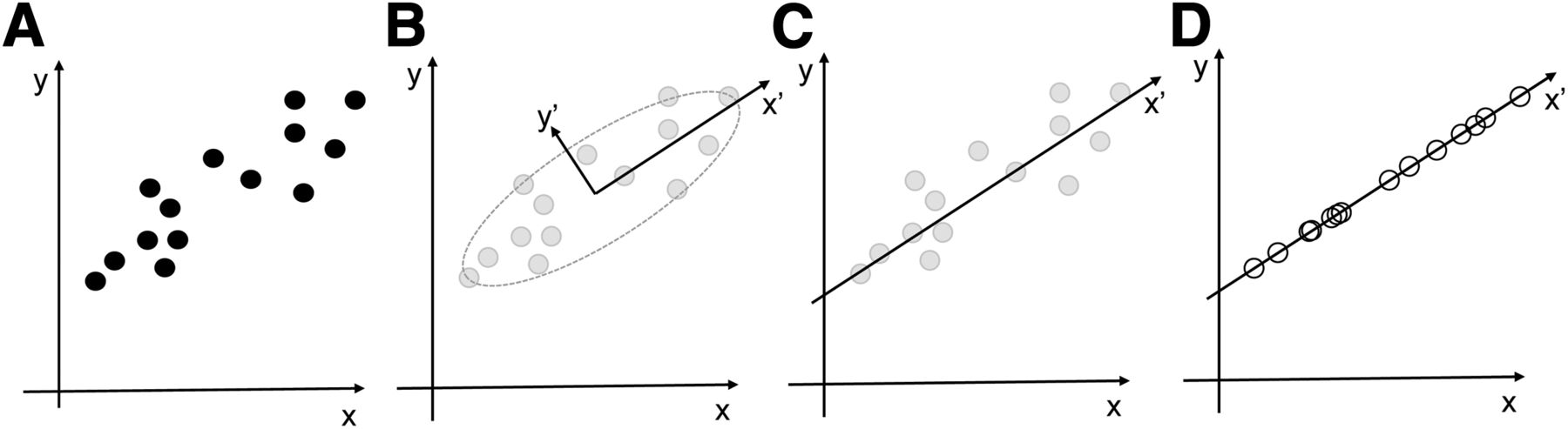
Illustration of principal component analysis. (A) Training dataset is shown as scatterplot. (B) Spread of data is greater along rotated axis x′ than y′. (C) Component y′ is removed since it is less important than x′. (D) Data points are moved to closest point along x′-axis; compressed (lossy) data is represented by measurement along x′, rather than using x and y.
K-Means Clustering (Fig. 6)
K-means clustering is an unsupervised algorithm for clustering data, where the term cluster refers to a collection of data points that are close to each other, for example, in terms of their measurements or feature values. K refers to the number of clusters and is specified by the programmer. The goal is to create K data clusters in which every data point is assigned to the cluster with closest resemblance. The computer does this through iteration: first, K cluster centers are chosen (i.e., random values are chosen for each feature); second, each data point is assigned to the cluster whose center is closest; third, the cluster centers are adjusted to be at the center of those data points that were assigned to them in step 2; and fourth, the process is repeated, starting at step 2 and ending when no data points change clusters. Given the random nature of initially choosing the center of the K clusters, it is possible to produce different solutions each time the program is run. To illustrate, amyloid brain PET scans could be clustered into K = 2 groups (e.g., amyloid-positive versus -negative) using known SUVR/ROI combinations for each scan. This, in turn, may suggest which SUVR/ROI combinations are most useful for clustering the scans. As another example, Blanc-Durand et al. used K-means clustering in 37 patients with 18F-fluoroethyltyrosine PET for newly diagnosed gliomas to suggest imaging features associated with progression and survival (24).

Illustration of K-means clustering. (A) Training dataset is shown as scatterplot (circles); stars indicate initial guesses for centers of 2 clusters. (B) Solid line midway between stars separates data into 2 clusters (gray and white). (C) Stars are moved to centers of each cluster. (D) Updated solid line midway between stars; 1 data point changes cluster. (E) Stars are moved to updated centers; because no data point changes cluster, algorithm converges.
Hierarchical Clustering (Fig. 7)
Hierarchical clustering is an unsupervised algorithm for clustering. Hierarchical clustering looks for data similarities by grouping nearest neighboring data points into pairs and clusters until no free data points remain. The resulting structure is referred to as a dendrogram. As an example, Tsujikawa et al. used a dendrogram to suggest related features on 18F-FDG PET in subjects with cervical cancer (25).

Illustration of hierarchical clustering. (A) Training dataset is shown as scatterplot. (B) Data points E and F are similar and are assigned to new cluster EF. (C) Nearest neighbors are G and EF (G is closest to point F within EF) and are grouped into EFG. (D) Data points B and C are similar and are assigned to new cluster BC. (E) Nearest neighbors are A and BC (A is closest to point C within BC) and are grouped into ABC. (F) Nearest neighbors are D and EFG and are grouped into DEFG. (G) Dendrogram indicates how clusters are hierarchically formed.
ISSUES TO CONSIDER
One of the questions that can be challenging is which ML algorithm to choose or why a certain algorithm has been used in a publication. To start off with, each ML algorithm targets a specific task (e.g., classification, regression, dimensionality reduction, or clustering). For instance, someone who wants to use an existing database of images and benign/malignant classifications to train an ML algorithm to classify future images might look to a supervised algorithm for classification, such as naïve Bayes classification, random forests, support vector machines, or CNNs. As it would be unlikely that the user would have a sense of the underlying probability distribution of the input data, a naïve classifier might be ruled out quickly. Next, the ML algorithm complexity, computational power, and predictive capability must be considered. For example, is it desirable to perform the work on a desktop workstation or will more computing power be needed? Indeed, to move forward, the user may try out each of the options to see which works best (using an available preprogrammed toolkit) or possibly reach out to someone with more of a theoretic grounding in ML about the next steps (e.g., a statistician, mathematician, computer scientist, or engineer—these people will often welcome your data with open arms!).
Another important consideration to take into account before selecting a complex ML algorithm, in addition to the potentially high computational cost, is overfitting, which is a situation in which the mathematic model too closely reflects minor variations in training data that are not predictive of validation and test data (e.g., when there is a lack of generalizability because the number of samples is too small). Consider, for instance, the data in Figure 5A; instead of unsupervised learning, had we seen this as a regression problem with y as the dependent variable, and had we tried to represent the data using an nth-order polynomial for an exact match, we would not necessarily have discovered the underlying (simpler and more representative) linear trend. A good model should be predictive and might not necessarily exactly reproduce the training data. Although a detailed analysis of the signs of overfitting and strategies to reduce it is beyond the scope of this paper, it is useful to know that some ML algorithms, for example, random forests, are more tolerant to overfitting.
This leads us naturally to the last issue in this article, namely the amount of data required to adequately train an ML algorithm, and the potentially high cost of acquiring sufficient data. As seen above, there are indeed ML algorithms that require very large datasets (especially when dividing them into training, validation, and testing subsets). However, many techniques have emerged to deal with this problem, including data augmentation. One pitfall is potential biases in datasets. In the early days of ML, there were ANNs unintentionally fooled by such innocuous issues as lighting conditions! The bottom line is that even the best augmentation techniques and the most tolerant ML algorithms will fail when subgroups are too small (which is, unfortunately, common in current radiology and nuclear medicine).
FUTURE PROSPECTS
Although ML has long existed, medical imaging applications are in their infancy (26). The advent of hybrid imaging (e.g., PET/MR) has brought enthusiasm to the field because this application is ideally suited for ML (in view of the different types of information that can be obtained simultaneously). However, several limitations remain. Typically, ML algorithms require large medical databases of sufficient quality to give reliable results. In March 2018, Thrall et al. suggested that AI medical imaging applications could benefit from “(1) national and international image sharing networks, (2) reference datasets of proven cases against which AI programs can be tested and compared, (3) criteria for standardization and optimization of imaging protocols for use in AI applications, and (4) a common lexicon for describing and reporting AI applications” (27). Standardization of imaging data acquisition is important because the scanner model and protocol used to acquire imaging data can influence radiomic features. Further, although initial results in ML are exciting, standardization and methodologic transparency are needed to deliver reproducible results and to speed clinical translation (28). Also, several topics require clarification as ML becomes ubiquitous in nuclear medicine, including the role of personal responsibility for patient care, fiduciary compact, data confidentiality, the need for bias-free algorithms, the process for validating ML algorithms, and the generalizability of results beyond a specific patient population for which data exist, to name a few. Further discussion on these topics is beyond the scope of this paper.
CONCLUSION
This article, the first in a 2-part series, has provided an introduction to ML in a nuclear medicine context. It has addressed the history of ML and described common algorithms, with illustrations of when these algorithms can be helpful in nuclear medicine. Part 2 will focus on current contributions of ML to our field, address future expectations and limitations, and provide a critical appraisal of what ML can and cannot do.
Footnotes
↵* Contributed equally to this work.
Published online Feb. 7, 2019.
Learning Objectives: On successful completion of this activity, participants should be able to (1) provide an introduction to machine learning, neural networks, and deep learning; (2) discuss common machine learning algorithms with illustrative examples and figures; and (3) compare machine learning algorithms and provide guidance on selection for a given application.
Financial Disclosure: Sandra E. Black received in-kind funding to her institution from GE Healthcare and Avid Pharmaceuticals. The authors of this article have indicated no other relevant relationships that could be perceived as a real or apparent conflict of interest.
CME Credit: SNMMI is accredited by the Accreditation Council for Continuing Medical Education (ACCME) to sponsor continuing education for physicians. SNMMI designates each JNM continuing education article for a maximum of 2.0 AMA PRA Category 1 Credits. Physicians should claim only credit commensurate with the extent of their participation in the activity. For CE credit, SAM, and other credit types, participants can access this activity through the SNMMI website (http://www.snmmilearningcenter.org) through April 2022.
- © 2019 by the Society of Nuclear Medicine and Molecular Imaging.
REFERENCES
- Received for publication November 14, 2018.
- Accepted for publication December 27, 2018.


