


Abstract
SPECT myocardial perfusion imaging has attained widespread clinical acceptance as a standard of care for patients with known or suspected coronary artery disease. A significant contribution to this success has been the use of computer techniques to provide objective quantitative assessment in the standardization of the interpretation of these studies. Software platforms have been developed as a pipeline to provide the quantitative algorithms researched, developed and validated to be clinically useful so diagnosticians everywhere can benefit from these tools. The goal of this continuing medical education article (part 1) is to describe the many quantitative tools that are clinically established and, more importantly, how clinicians should use them routinely in interpretation, clinical management, and therapy guidance for patients with coronary artery disease.
- quantitative LV perfusion
- quantitative LV function
- ischemic burden
- myocardial perfusion imaging
- transient ischemic dilation
- summed stress score
Nuclear cardiology encompasses measurements of myocardial perfusion, right and left ventricular (LV) function, synchrony of contraction, myocardial substrate metabolism, innervation, and inflammation. Nuclear cardiology is inherently digital and quantitative. The images are easily transformed into a digital pixel array. The scientific and clinical foundation of nuclear cardiology is also squarely framed in an extensive evidence base originating from the many books and thousands of articles published over the last 40 years (1). SPECT and PET imaging guidelines have also been published that describe the clinically established applications many of the quantitative parameters discussed (2,3).
This work, divided into 2 articles, is meant to be a snapshot in time of the state of the field of quantitative nuclear cardiology today. The purpose of the authors is 2-fold. In part 1, the goal is to describe the many quantitative tools that are clinically established. In part 2, the goal is to describe the tools that are evolving or emerging in nuclear cardiology. The secondary—albeit the most important—goal is for diagnosticians to use the established tools to improve the management of patients with heart disease and to learn about and anticipate the use of the evolving and emerging tools.
ESTABLISHED CLINICAL APPLICATIONS
Database Relative Myocardial Perfusion Imaging (MPI) Quantification
Perfusion Quantification
Quantification of myocardial perfusion extracted from the LV myocardium is one of the base modules incorporated into nuclear cardiology software packages. To perform this quantification, the 3-dimensional perfusion distribution is mapped to a standard template to eliminate the variability in LV size and shape between patients. The perfusion distribution is extracted from each LV short axis in the form of circumferential count profiles. The standard template is the 2-dimensional polar map (Fig. 1) that maps these count profiles into concentric rings from the base of the left ventricle (outer ring) to the apex (center of polar map) (4). Polar map distributions are computed in this manner for both the stress and the rest images from which estimates of stress-induced perfusion abnormalities can be identified and then further classified as ischemic or scar, using the rest map. The perfusion intensity in the most normal region within the LV is then used to normalize the polar map distribution to 100%. This produces a relative perfusion distribution, with each sector’s intensity being a percentage value relative to the uptake in the most normal myocardial region.

Method for polar map representation of LV myocardial perfusion distribution. (A) Circumferential count profiles are extracted from each short-axis slice from apex to base, depicted here as dashed circles (only 4 shown). (B) Circumferential profiles extracted from each LV short-axis slice plotted as normalized percentage counts extracted vs. angle around short axis for patient with hypoperfused septum. (C) Mapping of individual count profiles into rings, creating polar map.
With the relative perfusion map, one can use simple thresholds to identify regions of mild (e.g., <70%), moderate (e.g., <60%), and severe (e.g., <50%) hypoperfusion. This methodology assumes that the normal perfusion distribution is uniform throughout the LV myocardium. Unfortunately, there are several processes that introduce nonuniformities in the measured data—the most notable being photon attenuation—that result in reduction or misplacement of photons, thereby altering the measured distribution from the true perfusion distribution. The most prominent attenuation artifacts are breast artifacts, in which the soft tissue of the breast causes a decrease in counts in the anteroseptal region of the map, and diaphragmatic artifacts, in which the soft tissue of the diaphragm or torso causes a decrease in counts in the inferolateral region of the map.
Relative Versus Database Quantification
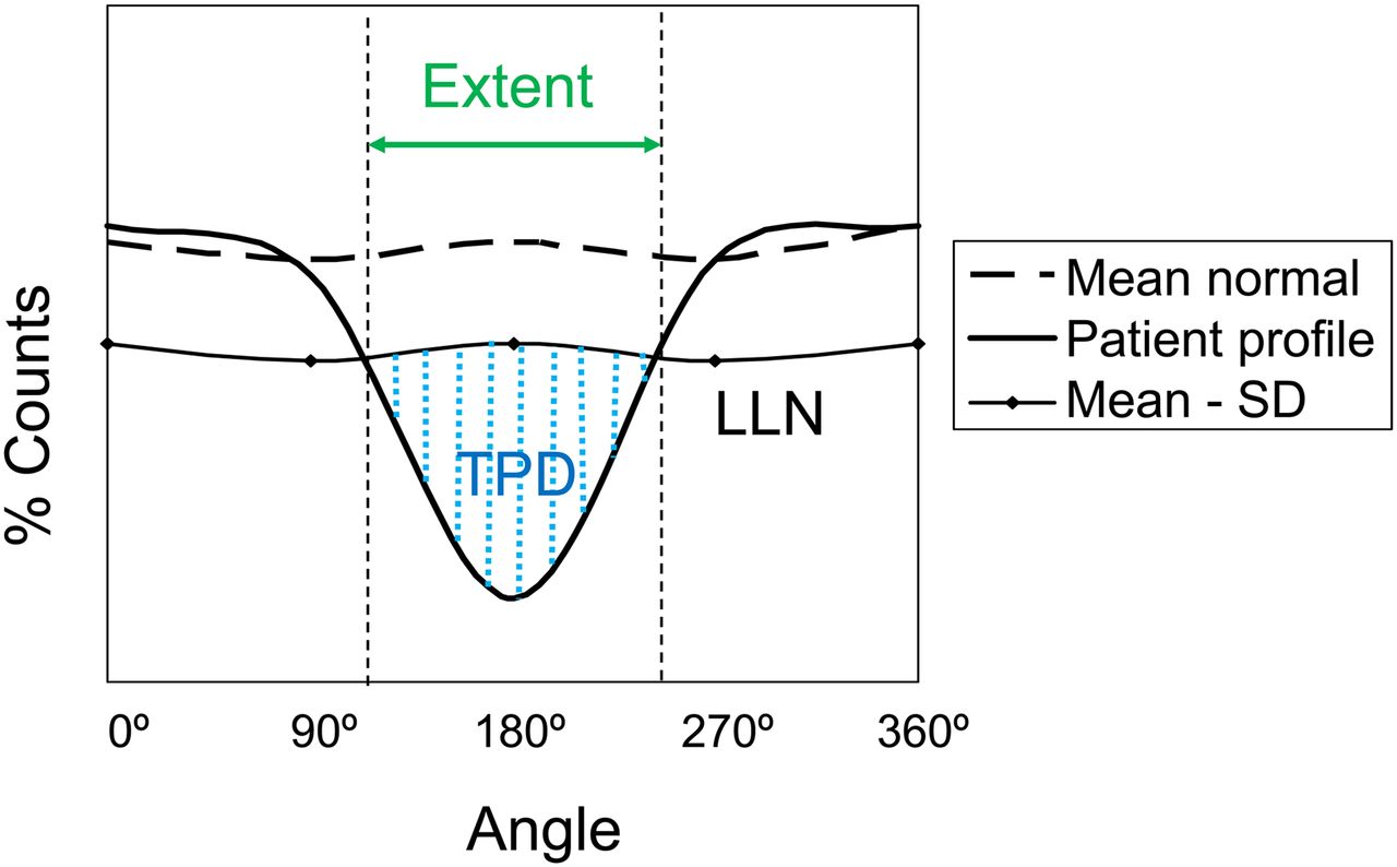
Photon attenuation is very dependent on body habitus and tissue density, which means that it can vary significantly between patients. To measure the regional effects on the perfusion distribution, polar map distributions are typically acquired from a population comprising age-matched patients with a low (≤5%) pretest likelihood of coronary artery disease (CAD). By averaging a large number (e.g., >20) of these distributions, estimates of the mean and its SD can be found for each sector in the polar map. A set of polar maps compiled in this manner is referred to as a normal perfusion database. Since the mean and SD are now estimated at each map sector, sector-specific thresholds based on a predefined number of SDs can be used. As an example, if a sector has a mean of 80% and an SD of 5%, one could use 2 SDs as the threshold for a mild defect (70% = 80% − 2 × 5%), 4 SDs for a moderate defect (60%), and 6 SDs for a severe defect (50%). This methodology is still the standard for perfusion quantification (Fig. 2) (5). It has the advantage of increased accuracy over uniform thresholds because it can account for attenuation effects when the studies are not corrected for attenuation, which is the norm for SPECT MPI.

Methods for detecting and measuring degree of hypoperfusion. Plot depicts how circumferential count profile is tested for abnormality. Patient’s normalized count profile (solid line) is compared against lower limit of normal (LLN) profile calculated as mean normal count response profile minus set number of SDs (usually 2–2.5). Extent of defect is given by angular range of count profile falling below LLN. Severity of deficit may be measured as sum of SD below mean normal profile for all abnormal angular samples. Total perfusion deficit (TPD) is marker of defect severity similar to SSS but measured for each sampled voxel, where each sample is scored from 0 (normal) to 4 (no uptake). Normal polar map generates TPD of 0, and maximally abnormal polar map (no myocardial uptake) would result in TPD of 100%.
Normal Perfusion Databases
Regional attenuation effects require the use of a normal database comprising human subjects with body habitus that matches test patients. For this reason, databases from North America, where the mean body mass index is around 30, should not be used in countries where the mean body mass index is significantly lower, for example, in Japan, where the mean body mass index is 22 (6). Other factors that influence attenuation effects are imaging position (supine, prone, upright) and photon energy; this means that matched databases should be used. The reconstruction algorithm also influences the estimated perfusion distribution, with the degree of smoothness dependent on the algorithm, filter, and number of iterations. One of the advantages of iterative reconstruction is that photon attenuation can be modeled and corrected for in the reconstruction process. When the proper modeling and corrections are applied, the measured distribution is a close match to the true perfusion distribution. In this case, databases can be used interchangeably between sex, patient populations, photon energy, and imaging position. This is more commonly seen in PET cardiac imaging.
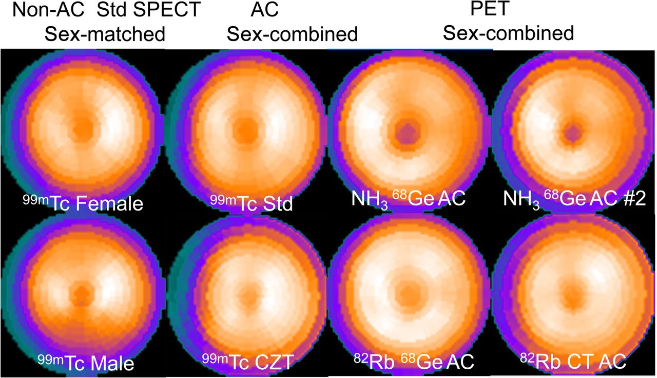
The latest generations of dedicated cardiac SPECT cameras and advanced iterative reconstruction software methods (7–11) have enabled meaningful reductions in imaging time and radiopharmaceutical doses (12–16). However, if the reconstruction parameters are not adjusted for increased noise in the reduced-dose/time images, it may be necessary to use normal databases that are “count-matched” to avoid bias induced by the noise mismatch between the normal database and the reduced-dose/time images (15–17). Another factor that affects the normal perfusion distribution patterns is camera technology; Figure 3 illustrates examples of the mean normal perfusion polar map differences in regional relative perfusion between SPECT and PET normal patterns, standard SPECT versus cadmium-zinc-telluride imaging, and attenuation correction versus studies not corrected for attenuation.

Comparison of different normal perfusion polar map patterns. Each of the 8 polar maps shown was generated from different patients with low likelihood of CAD as mean normal polar map relative response. Each normal pattern visually differs from the others. For example, attenuation-corrected (AC) normal pattern shows increased relative counts in inferior wall, compared with normal polar map from noncorrected perfusion studies. CZT = cadmium zinc telluride; Std = standard SPECT.
Segmental Perfusion Scoring
Visually identifying the location and severity of a perfusion abnormality was standardized to the 17-segment model in 2002, providing a simple template to score the severity (0 to 4: normal to absent) of the perfusion for the entire left ventricle (18). With the quantitative methods previously described using a normal database, thresholds can be mapped to each discrete severity score so that 17-segment regional scoring maps can be automatically derived. Segmental scoring is done for both the stress and the rest studies, providing a regional representation of lesion location, severity, and changes from stress to rest.
The segmental summed stress score (SSS) and summed rest score have been shown to provide significant incremental prognostic value for nuclear cardiology (19). Using the summed scores, one can derive the percentage of the left ventricle (%LV) at risk as a ratio of SSS and the maximum summed value [(68 = 17 segments × 4 maximum segmental score) × 100%], which is a severity-weighted estimate of total defect size. Figure 4 illustrates how an SSS of 18 is converted to 26% of the left ventricle hypoperfused. Since quantitative polar maps have several hundred sectors, compared with the simplified 17 segments, a more accurate estimate of defect size can be performed directly with the polar map using the continuous severity score and is most commonly referred to as the total perfusion deficit (20) (Fig. 2). The automation of total perfusion deficit and its severity-weighted %LV at risk provides one more quantitative measure to be used in nuclear cardiology for the detection and characterization of CAD. Table 1 lists established quantitative measures of LV perfusion and their threshold criteria for abnormality.
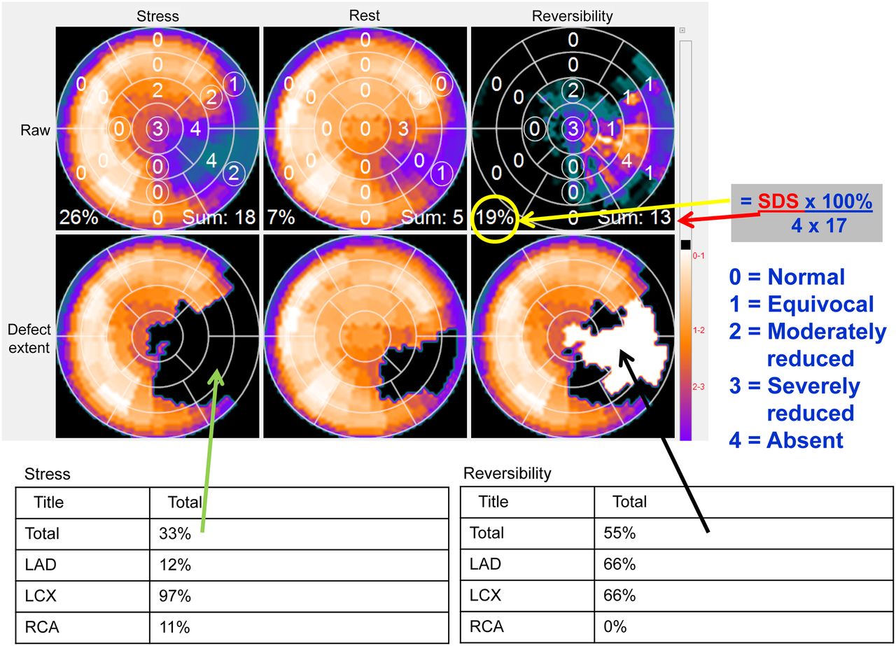
Methods for measuring degree of ischemic burden. Top row shows stress, rest, and reversibility polar maps scored (0–4) by computer algorithm using 17-segment model and their respective SSS, summed rest score, and SDS. SSS of 18 translates to 26% hypoperfused LV [=100% × 18/(4 × 17)]. SDS of 13 translates to 19% LV ischemic burden, which is greater than 10% threshold for patient benefiting from revascularization and thus candidate for catheterization. Second row shows same polar maps after they have been compared with traditional normal databases explained in Figure 2. Tables below show that defect extent (blackout polar map) is 33% of LV and that 97% of left circumflex (LCX) vascular territory is abnormal, as well as 12% of left anterior descending (LAD) and 11% of right coronary artery (RCA) territories. Reversibility polar map (whiteout) shows that 55% of stress perfusion defect improves at rest.
Quantitative Measures of LV Perfusion
Reversibility/Ischemic Burden
Reversibility
The term reversibility refers to the extent and magnitude of improved perfusion when the myocardium is at rest, compared with the myocardial hypoperfusion at peak stress. The general approach is to generate a reversibility polar map distribution calculated by normalizing the same region in the resting distribution to the most normal region in the stress distribution. Once normalized, the normalized stress distribution (expressed as 0%–100%) is subtracted from the normalized resting distribution and what remains are the areas of improved perfusion at rest, or the reversibility map. This myocardial reversibility distribution is then compared with normal limits to establish if the differences are statistically significant (Fig. 5) (21). In normally perfused myocardium, the mean normal reversibility is zero as no relative changes are expected. This approach has been validated in a multicenter trial (22). Although the degree of reversibility from MPI studies is due to relative changes in myocardial blood flow between stress and rest, it is commonly clinically considered the degree of ischemia. Direct imaging of myocardial ischemia can be achieved by imaging radiopharmaceuticals that are free fatty acid analogs and glucose analogs (23).

Method for detecting and measuring degree of defect reversibility. Plot depicts how circumferential reversibility profile is tested for improvement. Reversibility patient profile is generated by subtracting normalized stress count profile from resting count profile. Angular range that improves in relative perfusion from stress to rest is shown by increasing reversibility above zero. Mean normal reversibility profile hovers around zero since in healthy patients no relative perfusion change is expected between stress and rest. Angular extent of significant reversibility is depicted as portion of reversibility profile that jumps above upper limit of normal reversibility given by mean normal plus statistically determined number of SDs.
Another approach to quantifying reversibility is to use the summed difference score (SDS) (Fig. 4). The SDS is determined as the SSS minus the summed rest score. For purposes of risk stratification, the SDS is categorized as low (0–2), intermediate (3–7), or high (>7) (24).
Ischemic Burden
A more contemporary approach to measuring the degree of LV myocardial ischemia is the concept of ischemic burden. Quantification of this parameter relies on the SDS scores assigned using the 17-segment model (Fig. 4). The SDS score is converted to a global %LV ischemic burden by dividing the SDS by the maximum possible SDS score (a score of 4 × 17 segments = 68) and multiplying it by 100%. Figure 4 illustrates how an SDS of 13 is converted to a 19% LV ischemic burden. The reason this score has become popularized are the influential studies demonstrating that a cutoff of 10% LV ischemic burden differentiates those patients who would lower their risk of cardiac death after revascularization (≥10%) from those patients who would benefit more from medical therapy alone (<10%) (25,26). These findings imply that there has to be enough LV myocardium that is ischemic for an invasive procedure such as revascularization to reduce the risk of cardiac death to the patient.
Some clinicians use the stress %LV hypoperfused amount as a proxy for the %LV ischemic burden by converting the SSS score to %LV by dividing the SSS by 68 and multiplying by 100%. This substitution of SSS for SDS assumes that the reduction in counts at stress is completely due to ischemia. This assumption is true only when it is known that the patient has not had a previous myocardial infarction and that any potential attenuation artifacts have been accounted for by either attenuation correction or a combination of supine and prone imaging when using SPECT.
Infarct Size/Viability
Infarct Size
Quantification of infarct size with SPECT MPI uses the rationale that viable myocardial segments exhibit uptake of the perfusion tracer at rest whereas nonviable segments do not. The algorithm searches for the maximal counts in the entire LV myocardial distribution and identifies as nonviable those myocardial segments that fall below a percentage of this maximal value, usually 45%–50% when using 201Tl (27) and 60% when using for 99mTc perfusion agents (28). This measurement has been validated with many other measures of infarct size (29). Alternatively, the normal-database approach can be used for determining the rest defect, and this method was found to correlate well with infarct size defined by delayed enhancement MRI (30).
Viability
Measurements of infarct size by SPECT MPI are widely used, particularly in clinical trials. Yet, it is commonly accepted that SPECT MPI underestimates myocardial viability, particularly in patients with severe LV dysfunction (31). Glucose-loaded 18F-FDG PET imaging, particularly when combined with resting perfusion imaging, remains the reference standard for measuring myocardial viability (32,33).
Quantification of myocardial viability by combining resting MPI and a glucose-loaded 18F-FDG distribution relies on normalizing one distribution to the other before comparison. This normalization is done by first comparing the resting MPI distribution with an appropriate normal database. The hypoperfused areas can be identified by use of the normal database; the remaining normal areas are then used for normalization. The average count in the entire extent of normally perfused regions is computed for both the perfusion and the 18F-FDG studies. Then, the 18F-FDG distribution is scaled so that its average in the normal region is equal to that in the perfusion study. After normalization, the normalized perfusion distribution is subtracted from the normalized metabolism (18F-FDG) distribution. The difference between the distributions is expressed as a percentage of the normalized metabolism distribution. A threshold for this percentage difference can be set at any level (34), usually 5%–10%. Regions in the distribution that are above the threshold, and that have abnormal perfusion, are those that have relatively increased metabolism coexistent with relatively decreased perfusion. This region is known as the mismatch area. Any area above the threshold that is also abnormal for perfusion can be considered a mismatch consistent with myocardial hibernation and considered viable. If a myocardial region is statistically hypoperfused and the same region, in the 18F-FDG distribution, does not exceed the expected threshold for improvement, then these regions are considered to be matched and not viable. The extent of both viable and nonviable myocardium is quantified as %LV and, if the myocardial mass is computed, may be expressed in terms of grams of myocardial tissue. Although the presence of viable myocardium implies an increased likelihood of functional improvement with revascularization (32,33), there is currently a lack of consensus on the quantitative threshold of viable extent that would predict improvement, varying in different studies between 7% and 20% (35). This concept closely follows the concept of %LV ischemic burden explained above except that it is usually applied to patients with more advanced heart disease, such as heart failure.
Global LV Function
Global Functional Measurement
It is strongly recommended that electrocardiography gating be performed with all SPECT and PET protocols to allow assessment of multiple ventricular function parameters in addition to perfusion variables. Automatic computer-based methods quantify indices of global function, including LV ejection fraction (LVEF), end-diastolic volume, end-systolic volume, transient ischemic dilation (TID), myocardial mass, and diastolic function at stress and rest.
Quantitation of ventricular function and volumes with gated SPECT MPI can be performed by a variety of algorithms. The most common approaches are based on the automatic detection of endocardial and epicardial surface points across the cardiac cycle in 3 dimensions and may also consider the principle of constant mass across the cardiac cycle for improved robustness of the contour detection (Fig. 6) (36–39). In several independent studies (40–43) of LVEF obtained by SPECT MPI, the agreement between gated MPI and other standard measurements of LVEF has been shown to be very good to excellent, particularly when correlating LVEFs along a continuum from high to low values. Although LVEFs measured by different quantitative algorithms correlate highly, the specific cutoffs for abnormal LVEF may be method-dependent (43). For some methods, the normal threshold for the global LVEF measured by gated SPECT MPI images can be lower than that measured by other imaging modalities or by different algorithms. Unless the method uses Fourier temporal filtering (44), one of the reasons for the apparently lower LVEF is the use of only 8 gating intervals for binning the electrocardiography data. Recently, 16-frame gating has become more common in SPECT MPI, reducing the underestimation of LVEF. Normal limits for LVEF and LV volumes may depend on the sex of the patient, probably because of differences in absolute LV size in relation to SPECT image resolution, resulting in underestimation of end-systolic volume in patients with small hearts (45), particularly when end-systolic volume is less than 15 mL. Table 2 lists established quantitative measures of LV function and their threshold criteria for abnormality.
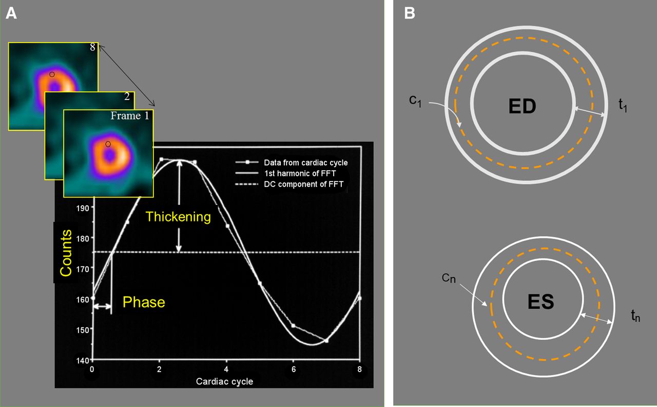
Method of detecting endocardial and epicardial LV boundaries for measuring global and regional function. (A) Maximal-count 3-dimensional sampling (c) of same LV myocardial region throughout cardiac cycle can be plotted as function of time (frame number) to extract percentage thickening throughout cardiac cycle. (B) Once end-diastolic (ED) 3-dimensional thickness (t) is determined (measured or assumed) to define endocardial and epicardial contours, change in maximal counts from ED is usually used to model how these contours move throughout cardiac cycle. These contours at ED and at end-systole (ES) are used to measure global LVEF, end-diastolic volume, and end-systolic volume. These same contour movements throughout cardiac cycle are used to measure mass, wall motion, and wall thickening, as well as diastolic function parameters. DC = average thickening for segment; FFT = Fast Fourier Transform.
Quantitative Measures of LV Function
Diastolic Function
Another group of parameters representing global ventricular function that can be obtained from MPI is diastolic function indices, in particular peak filling rate (PFR), defined as the greatest filling rate in early diastole. Diastolic function is traditionally assessed by echocardiography and gated blood-pool studies. PFR corresponds to the peak value of the first derivative of the diastolic portion of the gated frame curve (46) and can be normalized to end-diastolic volume, providing a clinically intuitive index. Additionally, time to PFR in milliseconds can be reported. Abnormality of LV diastolic function could be an early sign of CAD, congestive heart failure, and other cardiac conditions. The assessment of diastolic function has been shown to be feasible with gated SPECT MPI (47). When 16-frame gating is used, normal limits for PFR and time to PFR are similar to those reported with gated blood-pool studies. Agreement between SPECT and MRI in both PFR and time to PFR has been demonstrated when 32-frame gating is used for SPECT (48). Global time to PFR was shown to be less sensitive than regional parameters (49). Assessment of global diastolic function is not yet widely used, and the clinical value of MPI-derived diastolic function requires further evaluation.
Nonperfusion Parameters
In addition to perfusion defects, several nonperfusion characteristics can be observed with SPECT MPI, including mass (50), shape (51), and TID of the LV (52). Since contours of the LV are derived from gated and ungated scans, an estimate of the myocardial mass can be based on the volume between computed endo- and epicardial surfaces (53). Determination of endo- and epicardial surfaces requires that these 3-dimensional surfaces be generated by a computer algorithm such as with edge detection of the myocardium. The reproducibility of interobserver measurements for LV mass obtained from poststress MPI has been shown to be very high (54). LV mass derived by SPECT MPI also correlated with mass derived by CT; nevertheless, limits of agreement were wide, with lower values overestimated and higher values underestimated (54).
TID
Quantitative TID, in particular, has attracted clinical attention as an additional marker of high-risk disease derived by MPI. TID is usually calculated from the nongated rest and stress images as the ratio of LV cavity volume at stress divided by the volume at rest; however, the ratio can also be calculated from end-diastolic images obtained by gated SPECT (55). TID is considered present when the LV cavity appears to increase in the poststress images compared with rest images (52). This phenomenon may represent either apparent cavity dilation or subendocardial ischemia, which may explain why TID may be seen for several hours after stress, whereas functional abnormalities may no longer be present (Fig. 7). It appears that pharmacologically induced TID has prognostic implications similar to TID caused by exercise (56). Quantitative TID assessment has been shown to improve the detection of severe CAD when combined with perfusion assessment (55). The abnormality threshold for TID depends on the camera type, stress type, and imaging protocol used (57). A comprehensive comparison of abnormality thresholds for 8 different protocols (both exercise- and vasodilator-based) using data from 5 imaging centers from a large multinational registry, REFINE-SPECT (58), in 1,672 patients with a low likelihood of CAD and normal scan findings has been reported (58). The TID abnormality thresholds varied from 1.18 to 1.52 between various clinical protocols currently used (58,59). Protocols such as 82Rb, for which the stress perfusion images are acquired closer to peak stress, tend to yield a lower normal TID due to a reduction in the apparent LV chamber size at stress. TID upper limits have also been shown to be 1.15 for 82Rb PET MPI studies (60), lower than those for SPECT. This variability of TID across protocols underscores the importance of matching the TID limits to the specific MPI protocol used while integrating quantitative TID assessment to the clinical practice.

Method for detecting TID. (Top) TID due to change in LV cavity size dilated during stress as compared with smaller cavity size at rest. Blue ellipses depict hypothetical cavity size (in actuality done in 3 dimensions) to demonstrate difference between TID and transient subendocardial ischemia (TSI) and are not meant to be true detection of endocardial LV border. (Bottom) TID due to subendocardial ischemia during stress that normalizes at rest. Actual size of LV epicardium does not change from stress to rest. This is perhaps better named transient subendocardial ischemia. Cavity volumes at stress and rest are calculated in 3 dimensions from endocardial contours determined by computer algorithm.
Calcium Score
The use of hybrid SPECT/CT cameras allows for attenuation correction and for a more comprehensive assessment of CAD. Noncontrast CT images can be used for SPECT attenuation correction and, when electrocardiography-gated, for coronary artery calcium scoring (61,62). Both of these attributes have been shown to increase diagnostic performance (62). Because coronary calcium is pathognomonic of CAD, it can reclassify the risk and improve diagnosis in patients without known CAD who have normal findings on myocardial perfusion SPECT imaging. Moreover, the absence of coronary artery calcium (score of 0) is associated with a very low probability of future cardiovascular events (62). This information should be used to considerably lower the patient’s posttest probability of CAD and to increase the diagnostic confidence of the physician in excluding obstructive disease. Laboratories that measure the calcium score frequently report it.
Regional LV Function
Myocardial Thickening
Measurement of myocardial thickening is based on the observation that because of the limited spatial resolution of our imaging cameras compared with the myocardial thickness, a linear change in maximal counts in myocardial segments occurs as a direct response to a change in thickness (63) Thus, relative thickening is measured as a percent increase in maximal counts for each myocardial segment throughout the cardiac cycle. Even though gated MPI studies routinely use 8–16 frames per cardiac cycle, the temporal resolution of thickening is improved by the use of the Fourier transform (44). This mathematic step may be thought of as fitting to a sine wave the discrete counts from the same myocardial region in each of the 8 frames. Segmental thickening is then better approximated as the amplitude of the sine wave that was fitted to the counts from those regions. Quantitative programs display polar maps of regional (relative) thickening, often comparing it to a database of normal regional thickening. Average thickening by approximately more than 40% at the apex and more than 25% in the rest of the left ventricle is considered normal.
Myocardial Wall Motion
For measurement of myocardial endocardial wall motion, determination of the 3-dimensional LV endocardium is required. Determination of the endocardial boundary may be done using edge detection techniques, assumptions as to myocardial thickness, calibration to a myocardial phantom, or combinations of these.
Application of edge detection techniques to MPI studies is limited by the low spatial resolution of the nuclear imaging systems. The accuracy of this approach may be improved by calibrating against myocardial phantoms of known thickness. The other methods require a determination of the absolute myocardial thickness. The thickening method measures relative thickening rather than absolute thickness. One approach uses the myocardial location of the maximal count (corrected for scatter) to determine the midpoint of the myocardial wall segment (37,44). The assumption is made that at end-diastole the LV myocardial thickness is 1 cm, that is, 5 mm on either side of the midpoint. This defines the 3-dimensional endocardial and epicardial surfaces. It then uses the regional change in counts from the end-diastolic frame to determine the change in endocardial/epicardial surface location. For example, if at end-systole the myocardial counts in a segment double, the thickness will also double from 1 to 2 cm.
Myocardial Wall Thickening Versus Wall Motion
The use of myocardial wall thickening to express regional ventricular function has gained preferential status. The rationale is that the myocardium must thicken in order for the endocardium to have a meaningful wall motion. The endocardium may move without corresponding thickening, but this is due to either tethering to a region that is thickening or the torque of the heart. Neither of these 2 phenomena contribute to the stroke volume. Fully automated scoring of regional SPECT MPI LV wall motion and thickening can outperform experienced observers in the detection of CAD (64).
Diagnostic Performance of Established Applications
Diagnostic Performance
Relative quantification of SPECT and PET MPI has been extensively tested for diagnostic accuracy versus invasive angiography. MPI worldwide is performed mainly by SPECT (>90%). In a large clinical study of 995 patients, automated quantitative SPECT analysis was compared with visual analysis (65). A fully automated computer analysis of either attenuation-corrected or non–attenuation-corrected SPECT MPI data has been shown to be equivalent per patient and potentially superior for per-vessel analysis, when compared with expert analysis for the detection of stenoses of at least 70% based on angiographic criteria (66). The advanced methods allowing fully automated relative quantification were primarily optimized and validated for SPECT MPI. There are, however, equivalent tools available for relative perfusion quantification with PET. For PET, smaller studies quantitating MPI were performed also demonstrating high diagnostic accuracy (67).
Automation
The main advantage of computer-based relative quantification of perfusion over visual analysis is objectivity and reproducibility. Even expert physicians’ reading styles may differ, resulting in discrepancy in the subjective findings. Diagnostic agreement between 2 expert observers was found to be limited, with wide margins of error for the segmental summed scores (68). The reproducibility of software analysis is much better. In a study comparing visual and quantitative reproducibility of parameters obtained from repeated scans after a single injection, the quantification of perfusion deficit was found to have about half the variability of the intraobserver segmental scoring (same observer reading repeated in 3 wk) (69). Constant improvements in automatic processing allow reduced operator intervention and, consequently, further reproducibility improvements of the quantitative results, such as when all the available studies (stress, rest, gated, ungated) from the same patient study are processed in the same session
It has been demonstrated (70) that the repeatability coefficients of automatic perfusion quantification have been reduced to 2.6% and the failure rate for perfusion image analysis has been reduced to less than 1%. Techniques have been developed for the automatic flagging of the possible LV segmentation errors (71). Such methods allow processing of MPI images with minimal operator supervision, as was recently demonstrated in a large prognostic study (72).
Attenuation Correction and 2-Position Imaging
Automatic quantification can be performed either with or without AC (73). The analysis of most MPI AC studies shows significant improvement over non-AC studies in the specificity of detecting CAD (74). However, some groups (75) have attained only a modest improvement in diagnostic accuracy (by ∼3%) for perfusion quantification of attenuation-corrected images, as compared with noncorrected data. The use of AC for quantification of myocardial perfusion may eliminate the need for sex-specific databases (76). If attenuation maps are not available for correction, it is possible to use tomograms acquired from multiple patient positions (supine, prone, upright) to assess if a decrease in image counts is related to attenuation artifacts, since patient position alters attenuation artifacts (77). Quantitative techniques have been developed to estimate the size of perfusion defects simultaneously from 2 image positions—supine and prone acquisitions on conventional cameras (78,79) and upright and supine views on dedicated cardiac cameras (80). These quantitative techniques demonstrate improved prediction of obstructive disease by mitigating attenuation artifacts, similarly to attenuation-corrected analysis.
Quantitative Risk Prediction
The overall accuracy and precision of automatic analysis are critical for diagnostic purposes. The quantitative analysis could potentially be used directly for prognostic risk assessment (66,72,81). However, ultimately, the prediction of the relative benefit after therapy could be performed by quantitative rather than visual estimates of ischemia. Nevertheless, the validation studies to date of the ischemic defect size threshold for guiding therapy did not use the quantitatively determined %LV ischemic burden but rather relied on subjective visual scoring of the SDS converted to the %LV ischemic burden (26).
CONCLUSION
Quantitative clinical software tools in nuclear cardiology allow the objectification and standardization of measurements of cardiac perfusion, function, metabolism, innervation, and inflammation—a major strength of this imaging technique. Established tools are used clinically on a daily basis on most cardiac patients undergoing nuclear cardiology procedures to complement the diagnosticians’ acumen and to assist in study interpretation, clinical management, and therapy guidance.
Footnotes
This article is being jointly published in The Journal of Nuclear Medicine (DOI: 10.2967/jnumed.119.229799) and the Journal of Nuclear Cardiology (https://doi.org/10.1007/s12350-019-01906-6).
Learning Objectives: On successful completion of this activity, participants should be able to (1) know the basics of how quantitative parameters of relative left ventricular myocardial perfusion are measured and used clinically to differentiate patients with normal versus abnormal distributions; (2) know the basics of how quantitative parameters of left ventricular myocardial global and regional function is measured and used clinically to differentiate patients with normal versus abnormal function; and (3) describe and know how to use clinically nonperfusion quantitative parameters obtained from perfusion studies to modify the likelihood of the presence and extent of coronary artery disease in patients.
Financial Disclosure: Dr. Moody is an employee of Invia. Dr. Slomka receives grants from the National Institutes of Health and Siemens Medical Systems and receives software royalties from Cedars-Sinai. Dr. Germano receives royalties from most nuclear medicine companies. Dr. Ficaro is an employee of Invia. Dr. Garcia receives grants from Syntermed and GE Healthcare and receives royalties from Syntermed. The authors of this article have indicated no other relevant relationships that could be perceived as a real or apparent conflict of interest.
CME Credit: SNMMI is accredited by the Accreditation Council for Continuing Medical Education (ACCME) to sponsor continuing education for physicians. SNMMI designates each JNM continuing education article for a maximum of 2.0 AMA PRA Category 1 Credits. Physicians should claim only credit commensurate with the extent of their participation in the activity. For CE credit, SAM, and other credit types, participants can access this activity through the SNMMI website (http://www.snmmilearningcenter.org) through November 2022.
- © 2019 Society of Nuclear Medicine and Molecular Imaging & American Society of Nuclear Cardiology.
REFERENCES
- 1.↵
- 2.↵
- 3.↵
- 4.↵
- 5.↵
- 6.↵
- 7.↵
- 8.
- 9.
- 10.
- 11.↵
- 12.↵
- 13.
- 14.
- 15.↵
- 16.↵
- 17.↵
- 18.↵
- 19.↵
- 20.↵
- 21.↵
- 22.↵
- 23.↵
- 24.↵
- 25.↵
- 26.↵
- 27.↵
- 28.↵
- 29.↵
- 30.↵
- 31.↵
- 32.↵
- 33.↵
- 34.↵
- 35.↵
- 36.↵
- 37.↵
- 38.
- 39.↵
- 40.↵
- 41.
- 42.
- 43.↵
- 44.↵
- 45.↵
- 46.↵
- 47.↵
- 48.↵
- 49.↵
- 50.↵
- 51.↵
- 52.↵
- 53.↵
- 54.↵
- 55.↵
- 56.↵
- 57.↵
- 58.↵
- 59.↵
- 60.↵
- 61.↵
- 62.↵
- 63.↵
- 64.↵
- 65.↵
- 66.↵
- 67.↵
- 68.↵
- 69.↵
- 70.↵
- 71.↵
- 72.↵
- 73.↵
- 74.↵
- 75.↵
- 76.↵
- 77.↵
- 78.↵
- 79.↵
- 80.↵
- 81.↵
- Received for publication April 12, 2019.
- Accepted for publication July 11, 2019.


Jump to section
Related Articles
Cited By...
- No citing articles found.