


Abstract
We have developed a biventricular dynamic physical cardiac phantom to test gated blood-pool (GBP) SPECT image-processing algorithms. Such phantoms provide absolute values against which to assess accuracy of both right and left computed ventricular volume and ejection fraction (EF) measurements. Methods: Two silicon-rubber chambers driven by 2 piston pumps simulated crescent-shaped right ventricles wrapped partway around ellopsoid left ventricles. Twenty experiments were performed at Ghent University, for which right and left ventricular true volume and EF ranges were 65–275 mL and 55–165 mL and 7%–49% and 12%–69%, respectively. Resulting 64 × 64 simulated GBP SPECT images acquired at 16 frames per R-R interval were sent to Columbia University, where 2 observers analyzed images independently of each other, without knowledge of true values. Algorithms automatically segmented right ventricular activity volumetrically from left ventricular activity. Automated valve planes, midventricular planes, and segmentation regions were presented to observers, who accepted these choices or modified them as necessary. One observer repeated measurements >1 mo later without reference to previous determinations. Results: Linear correlation coefficients (r) of the mean of the 3 GBP SPECT observations versus true values for right and left ventricles were 0.80 and 0.94 for EF and 0.94 and 0.95 for volumes, respectively. Correlations for right and left ventricles were 0.97 and 0.97 for EF and 0.96 and 0.89 for volumes, respectively, for interobserver agreement and 0.97 and 0.98 for EF and 0.96 and 0.90 for volumes, respectively, for intraobserver agreement. No trends were detected, though volumes and right ventricular EFs were significantly higher than true values. Conclusion: Overall, GBP SPECT measurements correlated strongly with true values. The phantom evaluated shows considerable promise for helping to guide algorithm developments for improved GBP SPECT accuracy.
Gated blood-pool (GBP) SPECT offers several potential advantages over conventional equilibrium radionuclide angiography (planar ERNA). It has been shown that GBP SPECT assesses left ventricular (LV) ejection fraction (EF) more accurately than does planar ERNA (1). In addition, separating the ventricles and atria provides supplementary information regarding biventricular volumes, regional wall motion, and regional EF (2). Several automatic or semiautomatic methods have been developed that allow assessment of LV systolic function from GBP SPECT data (2–6).
However, relatively few GBP SPECT studies have dealt explicitly with validating right ventricular (RV) measurements (3–7). Yet, RV functional parameters may prove to be clinically quite important, considering that evidence has been mounting that RVEF may be a more sensitive predictor of adverse events than LVEF for some cardiac diseases, including congestive heart failure (8,9). Nevertheless, there have not yet been any reports published concerning the use of dynamic physical phantoms to evaluate algorithms that compute RV functional parameters. Therefore, we developed a dynamic cardiac biventricular phantom with which to evaluate new image-processing algorithms for the calculation of LVEF, RVEF, left ventricular volumes (LVVs) and right ventricular volumes (RVVs) derived from GBP SPECT data.
MATERIALS AND METHODS
Phantom Description
The phantom included 2 ventricular chambers. The LV consisted of 2 concentric ellipsoids forming inner and outer walls (Fig. 1B). The space between the 2 ellipsoids was filled with ultrasound acoustic gel, yielding a varying free wall and septal wall thickness varying between 0.5 and 1.5 cm. The gel is injected into the septal wall via 2 stopcocks embedded in the latex model. By keeping the injected volume of gel constant between the walls, ventricular wall thickness increased at systole (due to decrease of the ventricular inner volume) and decreased at diastole, thereby approximating systolic wall thickening. A realistic approximation of this situation is necessary for the evaluation of the possibility for the algorithm to separate both ventricles correctly during processing of the images. The relatively thinner (2 mm) single-walled crescent-shaped RV was attached to the outer septal LV wall and wrapped partway around the LV. Ventricles were cut off at the atrioventricular border, at the point at which the chambers were supplied by varying amounts of water from connecting plastic tubes to simulate LV and RV filling and emptying. An activity concentration of 370 MBq/L (10 mCi/L) of 99mTc in water was used in the chambers, with no background activity. Two separate piston pumps were used to supply the water to each ventricle, for which different stroke volume settings for both ventricles produced a wide range of simulated EFs and end-diastolic (ED) volumes. To set the ED volumes, the piston pump was fixed in its ED position. Valve 3 in Figure 1D was closed and volume was added or withdrawn to increase or decrease the ED volume. By changing the stroke length of the piston pump, stroke volumes could be controlled. After each individual experiment, volumes of both ventricles were measured at ED and at end-systole (ES) by suctioning out and measuring the contents of both ventricular chambers. To limit the necessary amount of radioactive tracer and not to contaminate the complete circuit, the ventricles were separated from the pump by 2 membranes, encapsulated in an acrylic housing (Fig. 1E).

Development and description of phantom. (A) Ventricles were cut off at atrioventricular border. (B) Single-walled RV was attached to double-walled LV. (C) Horizontal long-axis slice (top left), short-axis slice (top right), and vertical long-axis slice (bottom) of activity distribution in phantom. (D) Detail of biventricular model. Valves 1 are used to fill septal wall with gel; valves 2 are used to deaerate tubings, to inject tracer, and to empty ventricles for volume measurements. Valves 3 are in- and outgoing tubes to ventricles. (E) Overview of experimental model, with piston pump in back, membranes in middle, and ventricular model at front.
Data Acquisition, Reconstruction, and Reorientation
Twenty experiments were performed at Ghent University, for which RV and LV true volume and EF ranges were 65–275 mL and 55–165 mL and 7%–49% and 12%–69%, respectively. GBP SPECT data were acquired using a 3-detector gamma camera (IRIX; Marconi-Phillips) with low-energy, high-resolution collimators. Parameters of acquisition were as follows: 360° step-and-shoot rotation, 40 stops per head, 30 s per stop, 64 × 64 matrix, zoom 1.422 (pixel size, 6.5 mm), and 16 time bins per R-R interval, with a beat acceptance window at 20% of the average R-R interval. An R-wave simulator synchronized with the pistons supplied R-wave triggers. Projection data were prefiltered using a Butterworth filter (cutoff frequency, 0.5 cycle/cm; order, 5) and reconstructed by filtered backprojection using an x-plane ramp filter. Data were then reoriented into gated short-axis tomograms. Rectangular regions of interest, with outside masking, were drawn near simulated ventricles so that only ventricular structures and small portions of connecting tubes were visible. The resulting gated short-axis datasets then were copied to a CD-ROM, which was shipped to Columbia University.
GBP SPECT Algorithms
Processing was performed at Columbia University by 2 independent observers, who analyzed data without reference to each other’s results, and who had no knowledge of true phantom values. One observer reprocessed data >1 mo after his initial analyses without reference to his previous computations.
The algorithms used gated short-axis tomograms as input data. Algorithms ran automatically, and their first display to the observer was of a simultaneous view of RVV curves, functional parameters, and computed outlines superimposed on all short-axis and horizontal long-axis tomographic sections shown as a continuous cine loop. To produce these RV calculations, the programs first identified RV midplanes by searching for maximum count areas in volumetric regions likely occupied by these chambers. Counts above a 35% threshold of global maximum counts of the entire set of collected data were used to segment the RV from the LV. The same count threshold was used for both the RV and LV. The specific 35% count threshold value was chosen because it had been used successfully in previous studies to derive myocardial surfaces from myocardial perfusion gated SPECT and from GBP SPECT (7,10). Systolic count change images and Fourier phase images were used to estimate ED and ES tricuspid and pulmonary valve planes volumetrically. When presented with phantom data, the algorithms identified the posterior RV wall as the tricuspid valve plane and the anterior RV wall as the pulmonary valve plane. Moving tricuspid and pulmonary valve planes were interpolated from ED and ES valve planes for all other gating intervals. These planes were used to limit, in the posterior direction, the number of short-axis slices included in subsequent volume calculations. ED and ES vertical long-axis section count profiles were used to define moving pulmonary valve planes, so as to limit maximum heights of short-axis outlines.
Observers were free to accept all RV results or to modify intermediate choices. To allow this, observers reviewed identified mid-RV planes, indicated as boxes framing estimated midplane locations projected onto simultaneous cines of short-axis and vertical long-axis projections. ED and ES vertical long-axis and ED short-axis RV profile estimates were displayed, which observers could accept or redraw as necessary, until they were satisfied that generated RV outlines conformed to the visual impression of the size, shape, and motion of the RV throughout the heart cycle.
All RV counts were then subtracted from the 3-dimensional gated volume of count data, leaving primarily LV counts. These were handled by algorithms similar to those described above for the RV, again using 35% count threshold segmentation criteria. Automatically determined LV outlines superimposed on all short-axis and horizontal long-axis sections were then shown to an observer as an endless cine loop. As with the RV processing, observers were free to redraw ED and ES vertical long-axis and ED short-axis LV profiles, until they were satisfied that outlines conformed to the LV throughout the heart cycle. In general, for both RV and LV processing, manual interventions were rarely required for choices of ED or ES frames but usually were needed for vertical long-axis outlines for those simulations for which septal curvature was substantial, which was the case for more than half of the simulations. Volumes were computed geometrically from the number of 3-dimensional voxels corresponding to counts above the 35% count threshold, whereas EFs were computed from changes in counts summed over all included ventricular voxels. This “hybrid” approach was adopted because it had previously been found to provide optimal accuracy of calculations when compared with correlative MRI studies. These steps were accomplished using platform-independent computer-programming software (IDL; Research Systems Inc.) implemented on a commercially available computer system (ICON; Siemens Medical Systems).
Statistical Analysis
χ2 analysis was used to test whether data were normally distributed. Numeric results were reported as mean values ± 1 SD. In comparing algorithmic output to real phantom values, mean computed values were tabulated from 3 measurements: 1 each for the 2 observers, along with the 1 observer’s repeated measurements. In comparing computed volumes to true values, ED and ES volumes were considered together to form LVV and RVV datasets. Correlations between calculated and true values were expressed as the Pearson coefficient (r). Linear regression equations were calculated for all data pairs. Variability about the regression line was expressed as the SEE. Bland-Altman analysis of differences of paired values versus true values was used to search for trends and systematic errors. The limit of statistical significance was defined as probability P < 0.05 for all tests.
RESULTS
Calculation of Volumes
All values of both calculated and real EF and volume values were found to be normally distributed. Calculated ES and ED ventricular volumes of the 2 observers’ 3 analyses were averaged and correlated highly with real values (r = 0.95, P < 0.0001, n = 40 and r = 0.93, P < 0.0001, n = 40, for LV and RV, respectively) (Fig. 2). Bland-Altman analysis showed that, whereas slopes of trends were not statistically significant for left or right volumes (Fig. 2), nonetheless, the calculated LVV was statistically significantly higher than the real LVV and the calculated RVV was statistically significant higher than the real RVV. This was confirmed by paired t test results for both left volumes (109 ± 38 mL vs. 77 ± 34 mL; P < 0.001, n = 40) and for right volumes (143 ± 54 mL vs. 129 ± 50 mL; P < 0.01, n = 40). Subanalyses of ED volumes and ES volumes alone, rather than both ED and ES volumes analyzed together, yielded essentially the same results.

Linear regression and Bland-Altman analysis of mean calculated left and right ventricular volumes (MLVV and MRVV) vs. real left and right ventricular volumes (RLVV and RRVV).
Calculation of EF
Calculated LVEF and RVEF correlated highly with real values (r = 0.94, P < 0.0001, n = 20 and r = 0.80, P < 0.0001, n = 20, respectively) (Fig. 3). The difference in strengths of association (r = 0.80 for RVEF but r = 0.94 for LVEF) was not statistically significant for this sample size (n = 20). Bland-Altman analysis showed that slopes of trends were not statistically significant for LVEF or RVEF (Fig. 3). However, paired t test results showed that, whereas the calculated LVEF was the same as the real LVEF (40% ± 16% vs. 40% ± 16%; P = not significant, n = 20), the calculated RVEF was significantly higher than the real RVEF (38% ± 15% vs. 33% ± 12%; P < 0.0001, n = 20).

Linear regression and Bland-Altman analysis of mean calculated LVEF and RVEF (MLVEF and MRVEF) vs. real LVEF and RVEF (RLVEF and RRVEF).
Data Processing Reproducibility
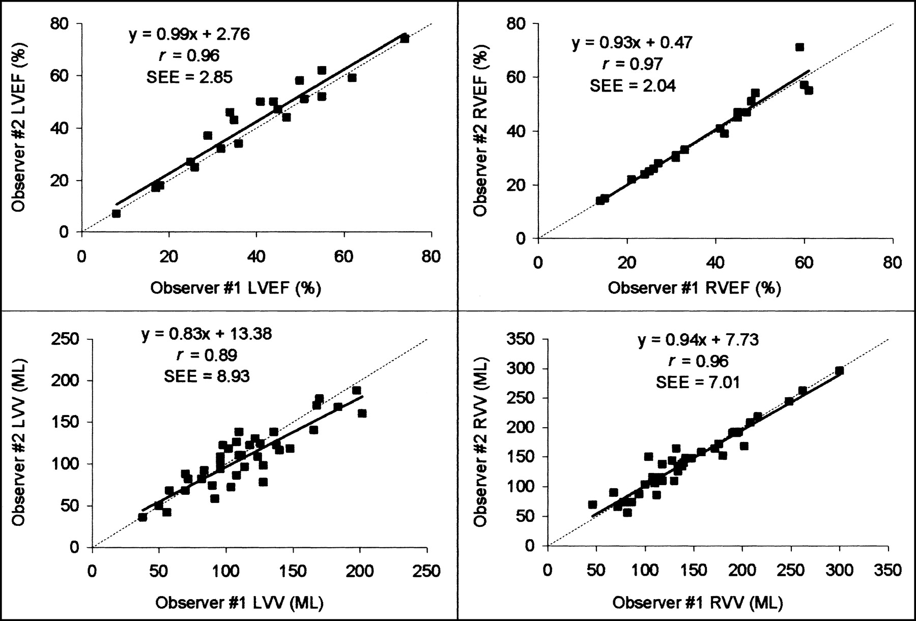
Correlations for LV and RV were 0.97 and 0.97 for EF and 0.89 and 0.96 for volumes for interobserver agreement (Fig. 4), and correlations were 0.98 and 0.97 for EF and 0.90 and 0.96 for volumes for intraobserver agreement (Fig. 5). All correlations were statistically significant (P < 0.0001). These values were consistent with those found in a previous validation of this algorithm against cardiac MR measurements (7).

Interobserver variability shown by linear regression of LVEF and RVEF and volume measurements of 2 different observers.

Intraobserver variability shown by linear regression of LVEF and RVEF and volume measurements of 2 observations for same observer.
Subanalyses of each of the 2 observers’ 3 measurements were not statistically different from analyses of the means of the 3 measurements, as expected, given the strengths of associations for interobserver and intraobserver agreement.
DISCUSSION
Overall, excellent correlation was obtained between computed versus real values for all measured parameters. However, the 6.4% RVEF SEE errors were larger than the 3.4% LVEF SEE errors. One factor contributing to this difference was that the phantom RV is wrapped around the LV for a greater degree of septal curvature than had been observed previously when applying the algorithms to patient data. Consequently, it was more challenging to the algorithms, and to the observers, to match regions to count thresholds for phantoms with the greatest amount of septal curvature. This may also have contributed to the larger RVV SEE of 9 mL compared with 5 mL for LVVs, although the larger range of real volume values (65–275 mL for RV but 55–165 mL for LV; Fig. 2) undoubtedly contributed to the finding.
Computed volumes were significantly larger than real volume values. This may have been due in part to the use of the 35% count threshold. Previous experiments by our group with dynamic ventricular phantoms showed that a count threshold of 50% yielded optimally accurate results, when experiments were performed with a variable background activity (11). A threshold of 35% may produce better agreement with MR for patient data, even though a higher threshold produces better agreement with phantom values, considering that the phantom lacked atria and a pulmonary outflow tract. Processing with a 50% count threshold should, in general, produce lower volume values than use of a 35% count threshold, which in the context of this investigation may have produced computed volumes in closer agreement with phantom values. Other investigators have found that the optimal threshold value for volume calculations derived from SPECT data can depend on the source shape; King et al. found that the use of a 50% threshold to determine the location of the edge of cylindric and spheric sources lead to a systematic, progressive underestimation of source volumes for ratios of diameter/full width at half maximum < 6 (12). That was the case in our experiments, and considering that the smallest RV dimensions of our phantom were 8 × 1.5 × 1.5 cm, partial-volume effects undoubtedly were an important factor in our experiments (13,14). Thus, it may well be that there is a need for using different thresholds for the RV compared with LV, given the different geometric shape of the RV compared with LV. Consequently, more realistic cardiac phantoms are warranted to clarify some issues, along with further correlative clinical studies with other imaging modalities, such as cardiac MR and x-ray contrast angiography.
There were several limitations to the study. Using algorithms developed for use with clinical data in phantom experiments can only give an estimate of the accuracy of the algorithms. Inclusion of background activity as well as use of different count thresholds and of different imaging parameters (e.g., different collimators, different image filters, 180° vs. 360° reconstructions) all may influence GBP SPECT volume computations. No corrections were applied for scatter or attenuation, which also may influence GBP SPECT calculations. The phantom itself was a simplified model of both cardiac ventricles, without atrial or vascular structures, background counts, or noncardiac scattering media. Identifying valve planes is an important part of processing GBP SPECT data, but this aspect of data processing was not realistically tested by the phantom used for this study. Nevertheless, to our knowledge, this is the first published report of the use of a dynamic physical phantom to evaluate the ability of GBP SPECT approaches to assess the RV and, as such, demonstrates that GBP SPECT algorithms can indeed produce realistic values of both RVVs and EFs.
CONCLUSION
We have demonstrated that the calculation of LV and RV ED and ES volumes of a dynamic cardiac phantom can be performed automatically by new GBP SPECT algorithms. Use of dynamic physical phantoms can help define the advantages and limitations of new algorithms that seek to measure both LV and RV functional parameters.
Acknowledgments
The authors thank Stefaan De Mey and Tom Cottens for their assistance with the phantom model experiments. This investigation was supported in part by a grant from Siemens Medical Systems, Inc. (Chicago, IL), Columbia University, and Syntermed, Inc. One of the authors (K.N.) stands to benefit from the sale of the software discussed in this article. This work was presented in part at the 49th Annual Meeting of the Society of Nuclear Medicine, Los Angeles, CA, June 15–19, 2002.
Footnotes
Received Sep. 30, 2002; revision accepted Jan. 21, 2003.
For correspondence or reprints contact: Pieter De Bondt, MD, Nuclear Medicine Division, P7, Ghent University Hospital, De Pintelaan 185, 9000 Ghent, Belgium.
E-mail: pieter.debondt{at}rug.ac.be


