


Abstract
Whole-brain activity is often chosen to quantitatively normalize peri-ictal and interictal SPECT scans before their subtraction. This use is not justified, because significant and extended modification of the cerebral blood flow can occur during a seizure. We validated and compared 2 automatic methods able to determine the optimal reference region, using simulation and clinical data. Methods: In the first method, the selected reference region is the intersection of peri-ictal-interictal areas with no significantly different z values. The other method relies on a 3-dimensional iterative voxel aggregation. The increase of the selected volume is stopped by using 2 different variance tests (Levene and SE). These algorithms were tested on 39 epileptic patients and were validated using 1 interictal and 10 peri-ictal scans simulated from the mean image of 22 healthy subjects. Results: In the patient studies, the mean relative activity of the selected regions, compared with whole-brain activity (classic normalization), was 122.6%. Their average relative size (compared with the size of the whole brain) was 33.2% for the z map method, 22.8% for the SE test, and 11.8% for the Levene test. After application of our automatic processes, subtraction of the simulated images revealed a recovery of abnormal regions up to 45% larger than the region obtained with classic normalization. Conclusion: These results illustrate the role of normalization on the subtracted peri-ictal and interictal images. Our methods are automatic and objective and give good results on various simulated images. The z map construction is worth considering because it is simple, selects large parts of the brain, and requires little computation time.
Brain imaging has become a mandatory step in the preoperative evaluation of refractory partial epilepsy. SPECT provides useful information about the location of the epileptogenic focus and is currently the only modality able to routinely provide information during the peri-ictal state. When the injection is given soon after seizure onset, the typical peri-ictal SPECT scan depicts a local increase in cerebral blood flow (CBF) well correlated with the location of the focus (1–3).
The sensitivity of the detection is, however, increased by building peri-ictal-interictal difference images, which aid identification of cerebral areas with significantly different CBFs between the 2 states (4–7). The construction of these subtracted images implies coregistration of the scans, quantitative normalization, voxel-by-voxel subtraction, and superimposition on MRI to improve spatial localization (8–11).
Quantitative normalization of images is of paramount importance because injected activities are not equal and global CBF can change during a seizure (12). The mean peri-ictal and interictal activities of the whole brain are often chosen to normalize the images (4,6), whereas some investigators prefer to choose the cerebellum (7). In a previous study (13), we showed that the choice of the whole brain was not the most relevant and that, for unilateral temporal lobe epilepsy, the contralateral lobe could be chosen as a reliable reference region. However, determining the lateralization of the focus is not always easy, and manually delimiting the reference region of interest (ROI) is long and tedious. Furthermore, in the case of extratemporal epilepsy, defining the areas unaffected by the seizure can be difficult because of the potentially large extent of the seizure network and the frequently low relative increase of CBF in extratemporal foci (3). In all cases, falsely localizing SPECT findings can lead to an inappropriate surgical decision (14,15).
Besides these points, the normalization step remains a subtle issue because the classic methods, as well as the new approaches, can be difficult to validate. The misunderstood phenomena underlying the epileptic pathology, and the unpredictability of its appearance, prevent us from considering any reference technique to be the gold standard.
In this study, we introduced and compared 2 automatic techniques able to find adequate reference regions for normalization. To evaluate the differences between classic normalization (by global brain activity) and our methods, we applied them to 39 patients whose refractory epilepsy was being evaluated before surgery. We also proposed a technical validation using simulated foci of various sizes and intensities added to the mean image of healthy subjects’ CBF scans.
MATERIALS AND METHODS
Patients and Image Acquisition
Interictal and peri-ictal SPECT scans were prospectively obtained for 39 patients (23 women, 16 men; mean age, 29 y) during presurgical investigation of their refractory epilepsy. Twenty-five patients had a unilateral temporal focus (left, 15; right, 10), 5 had a unilateral frontal focus (left, 2; right, 3), and 3 had bitemporal or multiple foci. These locations, deduced from deep-electrode implantation or postsurgical outcome, were not available for 6 patients still being evaluated.
Both scans were acquired after injection of 99mTc-ethylcysteinate dimer. The peri-ictal scan was acquired during video electroencephalographic monitoring, with the injection being administered as soon as possible after visual detection of the onset of electric (electroencephalographic) or clinical abnormalities. The peri-ictal and interictal images were acquired on a Prism 2000 (Picker International, Cleveland Heights, OH; 31 patients) or Varicam (Elscint Inc., Haifa, Israel; 8 patients) gamma camera with low-energy, high-resolution collimators. Both scans of each patient were acquired on the same machine. The images (128 × 128 voxel slices) were reconstructed with classic tools and filtering (Butterworth or Wiener).
Finally, the images were spatially coregistered with an algorithm maximizing their normalized mutual information, calculated from the joint histogram (11). In this step, the peri-ictal scan was defined as the target image, on which the interictal scan was shifted and reconstructed.
Simulated Data
To quantitatively evaluate the impact of normalization, we simulated 1 interictal and 10 peri-ictal scans with foci of known sizes and intensities (Fig. 1). Both kinds of images were built from the mean of 22 healthy subject scans obtained at the Department of Nuclear Medicine of the Queen Elizabeth Hospital in Adelaide, Australia. These examinations were acquired on a triple-head camera with ultra-high-resolution fanbeam collimators, after an injection of 99mTc-hexamethylpropyleneamine oxime, and were reconstructed as 91 transverse slices of 91 × 109 isotropic voxels (2 × 2 × 2 mm). These images are available in the Statistical Parametric Mapping software (Wellcome Department of Cognitive Neurology, Institute of Neurology, University College, London, U.K.).

Example of simulated SPECT images. (A) Interictal scan. Arrow shows 10% decrease of CBF in whole right temporal lobe. (B) One of 10 peri-ictal scans. Arrows show frontal and temporal hyperperfused areas.
Construction of Interictal Image.
In this mean image, we manually drew an ROI completely delineating the right anterior temporal lobe. Each voxel inside this temporal ROI was multiplied by 0.9 to model a 10% interictal decrease of CBF.
Construction of Peri-Ictal Images.
We first multiplied all the voxels of the mean image by 0.85 to simulate a lower injected activity. This step aimed at modeling the radioactive decay between the filling of the syringe and the injection time. Then, we drew a focus inside the temporal ROI about half its size. Each voxel of this focus was multiplied by 1.05, 1.1, 1.15, …, or 1.5, yielding 10 different peri-ictal scans with different increased temporal blood flows (+5%, +10%, +15%, …, or +50%). Furthermore, in each of these 10 scans, we added in the left frontal lobe (frontal ROI) a small ellipsis-shaped ROI with a 10% increase of CBF to simulate a remote activated area. The result gave the 10 simulated peri-ictal SPECT scans, each having the same frontal hyperperfusion and a different level of right temporal hyperperfusion. The size of the temporal ROI was 61.2 cm3 (7,650 voxels), and the size of the frontal ROI was 1.3 cm3 (168 voxels).
Noise.
Uncertainty was added to the simulated data by using a simple multiplicative process and our clinical images. Applying the formula of Budinger (16), we calculated the percentage of noise in each of the 78 SPECT scans included in our clinical study (2 scans for each of the 39 patients):
 where V is the number of voxels in the reconstructed brain and N is the total number of counts. The mean value in our set of 78 images was 13.5% (minimum, 9.3%; maximum, 18.3%). As a consequence, we multiplied each voxel value of the simulated images by a number randomly extracted from the set [−13.5%;+13.5%]. The aim of this step was to limit the smoothing effect caused by the construction of the initial mean scan from 22 real images, in order to provide more clinically realistic images.
Automated Search of Reference Area
z Map Approach.
As a first step, a common peri-ictal-interictal mask was built with a simple threshold (40% of the maximum count). The mean and the SD of the voxel values were then calculated within the mask in the peri-ictal and interictal scans, and each voxel value “i” was replaced by its z value. Finally, 2 z maps were constructed, in which each voxel represented the distance between its value and the mean activity, normalized by the global SD: z = |i − M|/SD, where M is the mean. We arbitrarily eliminated the z values higher than 1, in order to keep the areas with values close to the average CBF. The final reference region was the intersection of the z < 1 peri-ictal area and the z < 1 interictal area.
Voxel Aggregation Approach.
As for the previous method, a common mask was built, and the same threshold was used in order to start with an identical volume in both approaches. The principle of the technique relies on a 3-dimensional iterative voxel aggregation starting from a small volume (3 × 3 × 3 voxel cube), which we refer to as the seed point. The region stops increasing when a criterion, to be defined later in the text, is no longer verified.
Our algorithm contains 4 main steps. Let us consider the kth iteration. In step 1, the peri-ictal and interictal variances of the counts (Vpk and Vik, respectively) in the current kth region are calculated. In step 2, the Vpk and Vik are compared using a statistical test (the criterion to be defined later). In step 3, which is used if Vpk and Vik do not significantly differ, the current region is dilated and then steps 1 and 2 are repeated. In step 4, which is used if Vpk and Vik significantly differ, the algorithm is stopped and the region k − 1 is selected as the reference region.
The isotropic dilatation of the current region at each iteration was performed using simple morphologic mathematics tools (17). This kth volume was dilated by convolution with a simple structuring element, a 3-dimensional cross allowing intra- and interslice dilatation. Thanks to this growing process, the volume was iteratively thickened by a 1-voxel layer.
Comparison of Variances.
We chose to apply 2 different tests to compare the variances as a stopping criterion of voxel aggregation. The hypothesis was that if a region is not influenced by the seizure spread, its relative CBF distribution is not modified. Thus, we postulated that similar peri-ictal and interictal variances of the counts would indicate that the investigated area has no involvement in the seizure process and therefore could be chosen as a reference. We selected and compared the Levene test (18) and the SE test (13,19), both of which were elaborated to compare 2 variances (P < 0.05).
Final Choice of Reference Area.
Obviously, the result of this algorithm could depend on the seed point localization. To obtain a fully automated method, we regularly and automatically moved the seed point in the common mask (every 3 voxels in each direction). The final selected reference region was the largest obtained among all the regions born from each seed point.
Collected Data in Set of Patient Scans
The classic quantitative normalization process initially calculates both peri-ictal and interictal mean activities in the reference region and then equalizes these means to make the global peri-ictal-interictal CBF comparable. To be reliable, a reference region should be as large as possible, so that it is representative of the mean typical CBF. In addition, the mean value in such a reference region should be different from that of the global brain activity, especially when the peri-ictal and interictal scans vary considerably.
As a consequence, for each patient and for each method, the peri-ictal and interictal mean activities of the selected reference region, and its size, were calculated and then compared with the whole-brain activity and size. These 2 relative parameters were respectively referred to as ACTIV and SIZE and were compared using F tests.
Collected Data in Set of Simulated Scans
The aim of these computer-generated foci was to evaluate the effect of the different normalization choices on the subtracted images, because no reference is available in clinical images. We built the difference images by using a peri-ictal-interictal voxel-by-voxel subtraction after normalization, with the mean activities calculated by each of the 3 methods. The 2 ROIs identified by subtraction were then compared with their real sizes (7,650 and 168 voxels). The same was done using the classic normalization process, with the mean activity in that case calculated in the whole brain.
RESULTS
Figure 2 shows typical results obtained with each technique. For each of the 33 patients with well-defined epilepsy, the reference area never included the focus. For the other 6 patients, reference regions always excluded areas with evident peri-ictal and interictal abnormal CBF.

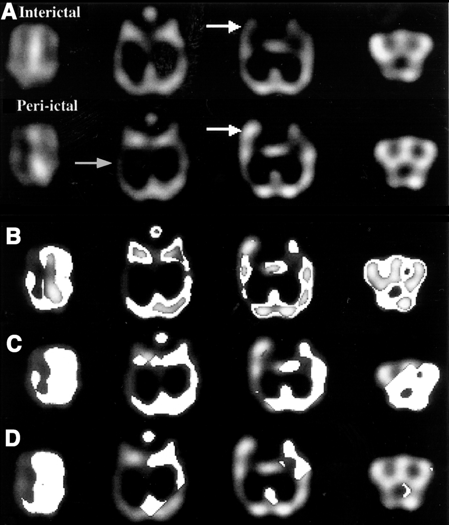
Typical example of selected reference region found by the 3 methods in patient with left temporal lobe epilepsy. (A) Original transverse slices in temporal orientation. Interictal images, at top, show decrease of CBF in left temporal lobe (white arrow). Peri-ictal images, at bottom, show global decrease of CBF in left hemisphere (gray arrow), except in temporal lobe containing focus and characterized by significant CBF increase (white arrow). (B) Reference regions (white areas) obtained with z map method. (C) Reference regions (white areas) obtained with Levene test. (D) Reference regions (white areas) obtained with SE test. In C and D, region boundaries sometimes look like lines because of cubic shape of seed point and symmetric shape of structuring element (3-dimensional cross).
Patient Data
Size of Selected Reference Area.
Table 1 shows mean, SD, SD/mean, and minimal and maximal SIZE parameters for the 3 methods. The size of the reference area never reached the size of the whole brain, the largest value being 42.8%. This point demonstrates that systematically, some areas in the brain (in fact, those with a high or a low CBF compared with global CBF) were not included in the reference region. Table 1 also shows that the z map method provided larger reference areas (the mean size being 33.2%, vs. 22.8% and 11.8% for the aggregation approaches) and more homogeneous results (the SD/mean value being 0.1, vs. 1.1 and 0.4 for the other 2 methods).
SIZE Parameter: Size of Selected Region Compared with Size of Whole Brain
Calculated Mean Activities in Selected Reference Area.
The calculated activities in the reference region found by the algorithms, compared with the whole-brain activity (ACTIV parameter), are presented in Table 2. These calculated values were always higher than 100%, implying that the mean activity in the regions was higher than the global brain activity.
ACTIV Parameter: Activity in Selected Reference Region Compared with Activity in Whole Brain
Data Analysis Using Fisher Statistics.
The aim was to evaluate the significance of the differences between the parameters calculated from the 3 methods.
For SIZE parameter values, the methods were compared 2 by 2. The results were F = 18.0 (P < 0.001) for Levene versus SE, F = 24.6 (P < 0.001) for z map versus SE, and F = 103.6 (P < 0.001) for z map versus Levene. The z map and the aggregation approaches gave regions of very different size. The 2 aggregation methods provided more comparable results, even if still significantly different.
For ACTIV parameter values, the results for the interictal and the peri-ictal sets, respectively, were F = 23.0 and 17.8 for z map versus SE (P < 0.001), F = 16.9 and 19.8 for z map versus Levene (P < 0.001), and nonsignificant for Levene versus SE. Thus, the 2 aggregation methods gave areas with comparable mean activities, whereas the z map technique provided results different from those of either of these methods.
Simulated Data
Table 3 shows the volume of the regions revealed by subtraction, compared with the actual volume of the regions of interest (7,818 voxels). Values are given for our 3 methods and for the classic normalization method, applied on the 10 peri-ictal scans. Figure 3 also presents the percentage of region recovery but separates the results obtained for the frontal and temporal ROIs.

Percentage of simulated ROI retrieval for frontal ROI (A) and temporal ROI (B). Curves represent size of areas revealed by subtraction, compared with actual size of simulated ROIs. Results were obtained after normalization by our automated processes and by classic method (whole brain).
Volume of Areas Obtained by Subtraction Compared with Actual Volume of ROIs (7,818 Voxels)
These data show, first, that the volume of the abnormal regions revealed by our methods was always higher than the volume of the abnormal regions revealed after global normalization; second, that for all methods, volume decreased when temporal focal activity reached +35% or more; and third, that this decrease was significantly larger with the global normalization method than with our methods. For the +50% focus, our methods revealed 76.1% of the real regions of interest whereas the classic process revealed only 40.1% of the information. The difference was even larger with the frontal ROI only—57.2% versus 12.4%.
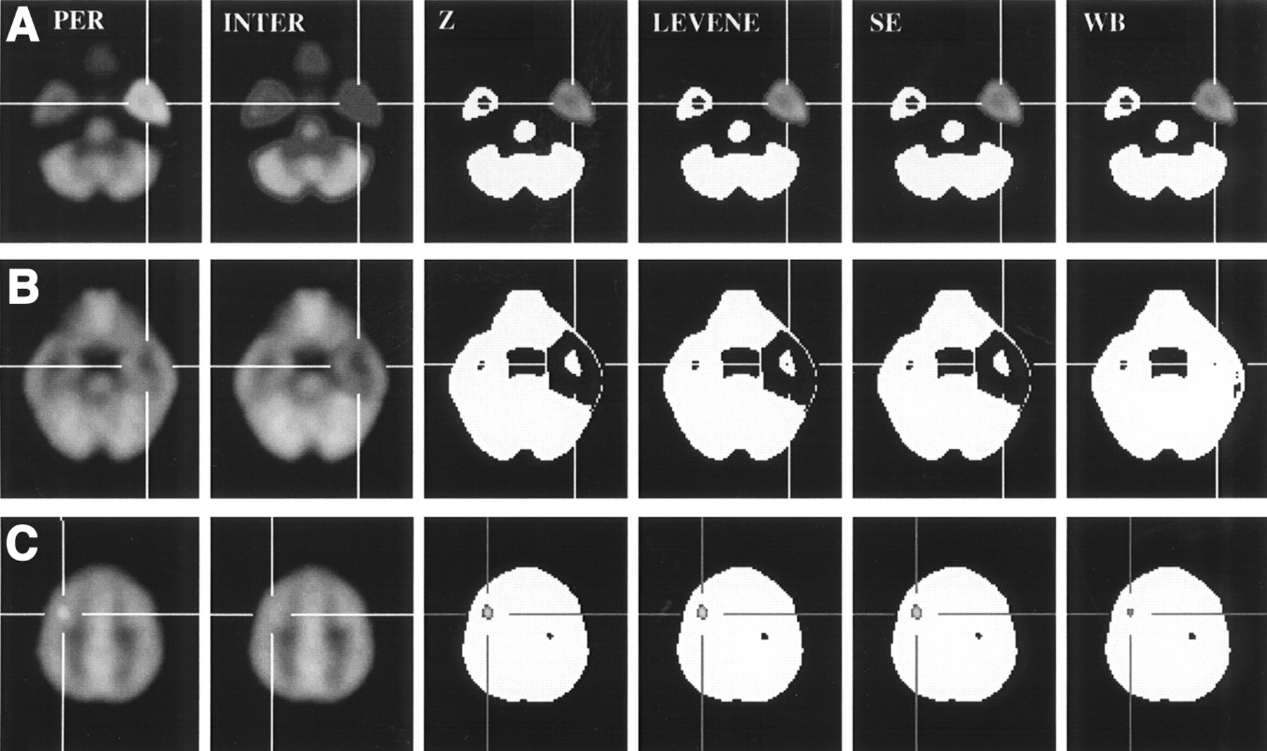
As an illustration, Figure 4 shows subtraction of the interictal scan from the +50% peri-ictal scan, as obtained with our methods and with the classic normalization process. The temporal focus was correctly revealed by all methods (Fig. 4A), including classic normalization. However, our methods revealed the complete extent of the interictal temporal CBF decrease—an extent that was not revealed using the classic process (Fig. 4B). Furthermore, our techniques exposed a larger part of the frontal focus (Fig. 4C).

Subtraction of +50% peri-ictal and interictal simulated images. From left to right, images are peri-ictal scan (PER); interictal scan (INTER); and abnormal regions retrieved after z map (Z), Levene (L), SE, and classic (whole brain [WB]) normalization methods. Results are shown for pole of right temporal lobe (peri-ictal, +50% increased CBF; interictal, −10% decreased CBF) (A), for higher slice of right temporal lobe (peri-ictal, normal; interictal, −10% decreased CBF) (B), and for left frontal lobe (peri-ictal, +10% increased CBF; interictal, normal) (C).
Lastly, Figure 5 illustrates the gain of volume recovery obtained by subtraction with our methods compared with the results of the classic process. This figure shows that our techniques can reveal up to 45% larger areas.

Recovery improvement in each subtracted image for frontal ROI (A) and temporal ROI (B). Curves represent difference between size of regions revealed by our methods and size of regions revealed using classic normalization.
DISCUSSION
The aim of the peri-ictal-interictal difference images is to underline the cerebral areas in which CBF differs between the interictal state and the peri-ictal state. These subtracted images improve the localization of the epileptic focus (4,5) essentially because they avoid the uncertainty due to subjective visual comparison of scans. Traditionally, the whole brain is chosen to calculate the mean peri-ictal and interictal activities that will further be used to normalize the scans. But in epilepsy, large, distant, and numerous areas can be involved during a single seizure, and the CBF increase in such regions may be quite high. Therefore, the choice of the whole brain is controversial, because pathologic CBF variation of cortical areas implicated in the underlying pathology is included in the calculation of normalization activity (13).
The aim of our normalization methods was to give the process more objectivity and to automatically find areas that had no significant CBF variation and were large enough to be representative of the global and standard CBF. The automatic approach was chosen to suppress the subjective steps such as ROI drawing or whole-brain selection.
In z map construction, we chose a z < 1 threshold to eliminate extreme values of CBF in the normalization process. The size of the selected area was then about 33% of the whole brain (Table 1). This arbitrary choice, which was made after several trials, seemed to be the most acceptable choice after a visual analysis of the selected regions. The threshold appeared to be a good compromise between the rejection of high and low CBF areas and the selection of sufficiently large reference regions, as illustrated by Figure 6. This figure shows that for a z < 2 threshold, the SIZE parameter becomes high, increasing the risk that activated areas will be taken into account, whereas a z < 0.5 threshold can lead to the selection of reference regions that are too small (less than 20%).

Influence of z threshold on SIZE parameter. Top curve is for patient with maximum SIZE parameter, bottom curve is for patient with minimum SIZE parameter, and middle curve is mean SIZE for whole set of 39 patients.
An advantage of the z map method is the rapidity of detection, which takes 5 s, compared with the 15 min required for voxel aggregation. Therefore, this technique is better adapted for clinical use. The calculation in the aggregation process is long because every 3-voxel increment in every direction is successively chosen as a seed point. This systematic test is, however, fundamental because the aggregation process is origin dependent.
In other respects, our results show that the 2 tests of variance do not provide similar results. The Levene test is known to be more robust than the SE test when large samples are studied, but the Levene test gives mediocre results for small samples. This point may explain why voxel aggregation with the Levene test sometimes stops with very small areas (Table 1). Thus, a conceivable improvement would be a strategy of combining both tests, with the Levene test being used only after the region has reached a given size.
The use of our algorithms on the simulated peri-ictal and interictal images emphasizes the weight of the normalization process on the difference images and justifies an accurate choice of reference region. After subtraction, our normalization methods underlined areas up to 35% larger than those obtained with the classic process (temporal ROI). The gain of data was even higher with the frontal ROI: +45% (Fig. 5). This means that these automated approaches allow the retrieval of a greater number of abnormal regions than does classic normalization, because the automated approaches detect areas of small spatial extent or of little CBF variation, particularly when the peri-ictal scan contains an intense focus (Fig. 4). This capability is important if one wants information about the spread of ictal abnormalities, mainly if the ictal injection occurred too long a time after the beginning of the crisis.
Our simulated images were constructed from hexamethylpropyleneamine oxime reference data. Even if a slight difference in normal distribution exists with ethylcysteinate dimer (20), its results should be identical because of the important peri-ictal and interictal CBF modifications compared with the normal areas.
At last, to improve validation, we could consider the use of a phantom or a computed simulator modeling the SPECT reconstruction. In addition, a larger clinical study could be performed, because our preliminary results (39 patients) agreed with our initial hypotheses. For instance, the calculated mean activity in a selected reference area should always be higher than the mean activity in the whole brain, because the labeled molecule is less taken up in the white matter than in the cortex and because the signal is lower in the deep brain structures because of attenuation. Our results agreed with this statement because they showed a significant increase in the ACTIV parameter.
Furthermore, in all patient studies the reference regions were smaller than global brain size—a satisfactory result considering our initial requirements. However, this point cannot lead to a definitive clinical validation, because as long as we do not understand the whole epileptogenic process, it remains problematic to evaluate our quantitative results without a reference methodology.
CONCLUSION
The 2 methods we have described increased the sensitivity of focus detection by subtraction SPECT, thanks to normalization improvement. The main interest of our study was the increase in objectivity brought about by automation of the process. Furthermore, the results obtained from the simulated data established the degree of confidence that one can give to the clinical results. Lastly, these approaches can be applied at any other functional imaging investigation involving 2 different cognitive or pathologic states requiring normalization and comparison.
Footnotes
Received Dec. 7, 2001; revision accepted Jul. 5, 2002.
For correspondence or reprints contact: Nicolas Boussion, PhD, Hôpital Notre-Dame, Pavillon J.A. de Sève (local Y-1619), 2099 Alexandre de Sève, Montréal, Québec, Canada, H2L 2W5.
E-mail: nicolas.boussion{at}umontreal.ca


