


Visual Abstract

Abstract
Estimation of the time-integrated activity (TIA) for dosimetry from imaging at a single time point (STP) facilitates the clinical translation of dosimetry-guided radiopharmaceutical therapy. However, the accuracy of the STP methods for TIA estimation varies on the basis of time-point selection. We constructed patient data–driven regression models to reduce the sensitivity to time-point selection and to compare these new models with commonly used STP methods. Methods: SPECT/CT performed at time period (TP) 1 (3–5 h), TP2 (days 1–2), TP3 (days 3–5), and TP4 (days 6–8) after cycle 1 of [177Lu]Lu-DOTATATE therapy involved 27 patients with 100 segmented tumors and 54 kidneys. Influenced by the previous physics-based STP models of Madsen et al. and Hänscheid et al., we constructed an STP prediction expression, TIA = A(t) × g(t), in a SPECT data–driven way (model 1), in which A(t) is the observed activity at imaging time t, and the curve, g(t), is estimated with a nonparametric generalized additive model by minimizing the normalized mean square error relative to the TIA derived from 4-time-point SPECT (reference TIA). Furthermore, we fit a generalized additive model that incorporates baseline biomarkers as auxiliary data in addition to the single activity measurement (model 2). Leave-one-out cross validation was performed to evaluate STP models using mean absolute error (MAE) and mean square error between the predicted and reference TIA. Results: At days 3–5, all evaluated STP methods performed very well, with an MAE of less than 7% (between-patient SD of <10%) for both kidneys and tumors. At other TPs, the Madsen method and data-driven models 1 and 2 performed reasonably well (MAEs < 17% for kidneys and < 32% for tumors), whereas the error with the Hänscheid method was substantially higher. The proof of concept of adding baseline biomarkers to the prediction model was demonstrated and showed a moderate enhancement at TP1, especially for estimating kidney TIA (MAE ± SD from 15.6% ± 1.3% to 11.8% ± 1.0%). Evaluations on 500 virtual patients using clinically relevant time–activity simulations showed a similar performance. Conclusion: The performance of the Madsen method and proposed data-driven models is less sensitive to TP selection than is the Hänscheid method. At the earliest TP, which is the most practical, the model incorporating baseline biomarkers outperforms other methods that rely only on the single activity measurement.
For neuroendocrine tumors, [177Lu]Lu-DOTATATE peptide receptor radionuclide therapy (PRRT) is typically administered over the course of 4 cycles at 7.4 GBq/cycle (1). In addition to the therapeutic β-particles, 177Lu emits imageable γ-rays, which provide a unique opportunity to perform imaging-based dosimetry after each cycle to plan subsequent cycles. Despite this potential, fixed-activity protocols without any dosimetry-guided adjustments remain the standard of care in [177Lu]Lu-DOTATATE PRRT and some other radiopharmaceutical therapies.
Dosimetry-guided treatment planning is rarely used in routine radiopharmaceutical therapy clinical practice, lagging external-beam radiotherapy, for which substantial time and resources are used to generate individualized plans. In radiopharmaceutical therapy, pharmacokinetics can vary considerably between patients; hence, multiple-time-point imaging is desirable to determine the time-integrated activity (TIA) for dosimetry. Imaging typically takes place over a few days to 1 wk, depending on the effective half-life (Teff) of the agent, requiring multiple return visits that can be burdensome and costly. Furthermore, SPECT data acquisition is relatively time-consuming, especially if multiple bed positions are necessary. With the goal of simplifying dosimetry, Madsen et al. (2) and Hänscheid et al. (3) derived equations for estimating TIA from an activity measurement performed at a single time point (STP). Their methods are based on the principle that the TIA can be computed exactly from a single activity measurement, A(t), at time t, assuming monoexponential clearance, as  . Because the Teff is typically unknown for a new patient, the method of Hänscheid et al. (3) assumes that
  1, simplifying to the closed form,
  . This approximation presumes that the imaging time point is near the unknown Teff. The method of Madsen et al. (2) does not require an assumption about the time point but instead requires prior knowledge of the population average Teff, Teff,p, which is then used directly in the equation
  . A challenge with STP estimation of TIA is the selection of the optimal timing of the measurement, which varies depending on the pharmacokinetics associated with each therapy and tissue type. For [177Lu]Lu-DOTATATE therapy, previous studies (3–5) reported the optimal sampling time to be about 3 d for kidneys and 4–5 d for tumors because of the longer Teff associated with the latter. However, in practice, imaging close to that time may not always be feasible because of patient and clinic schedules. Earlier imaging, ideally on the same day as therapy, is most suitable when considering patient convenience and clinic logistics.
Our study is motivated by the value of STP methods that are less sensitive to time-point selection. Having access to retrospective multiple-time-point SPECT/CT imaging data after [177Lu]Lu-DOTATATE PRRT in a cohort of 27 patients (54 kidneys, 100 tumors), we had a goal of constructing and evaluating data-driven regression models for estimating TIA from a single activity measurement. We also strove to develop a model incorporating additional clinically relevant baseline data ([68Ga]Ga-DOTATATE PET SUV and laboratory biomarkers; Fig. 1). Such imaging and nonimaging biomarkers have been investigated as predictive and prognostic factors in 177Lu therapies (6,7), but to our knowledge, they have not been investigated in the context of reduced-time-point imaging. Using the TIA calculated from multiple-time-point SPECT/CT as the reference standard, we evaluated the performance of our proposed regression models and compared this performance with that of previous STP methods.

Proposed data-driven models use either single activity measurement or single activity measurement plus biomarkers to predict TIA. Reference TIA is calculated using multiple-time-point 177Lu SPECT/CT imaging. HU = Hounsfield units.
MATERIALS AND METHODS
Data-Driven STP Model Derivation (Model 1)
If we assume biexponential behavior for the kinetics of the radiopharmaceutical in the tissue of interest, the activity at time t, A(t), can be expressed as Eq. 1where
  is the scale parameter,
  is the effective decay rate, and
  is the effective absorption rate. Then the TIA is
 Eq. 2
Eq. 2
Inspired by the STP models discussed previously, we proposed a group of prediction models with a more generalized functional form: Eq. 3where
  is a function of measurement time, t. Therefore, the Hänscheid and Madsen methods are both special cases under this framework, with
  and
and  . Rather than these parametric functions, we used a nonparametric generalized additive model (GAM) (8) to estimate the optimal
  in a data-driven manner, minimizing the normalized mean square error (MSE) between the predicted TIA and the reference TIA, which we consider to be the integral of the time–activity curve from multiple-time-point imaging. We used normalized least squares as our objective function rather than ordinary least squares to avoid overweighting the few patients with very high TIA values.
The GAM is able to fit nonlinear trends with multiple basis functions. It is entirely data-driven, without any model assumption such as exponential kinetics. Our proposed model is thus a nonparametric smooth curve, which gives a consistent prediction at any time by directly minimizing the prediction error. The prediction is fitted with a local estimation in a data-driven way, which means the prediction for an individual is based on other patients with activities measured at similar times.
STP Model Extension: Incorporating Auxiliary Data (Model 2)
We then fit another data-driven model (model 2) that, in addition to the single activity measurement, can incorporate auxiliary data to potentially improve TIA prediction (Fig. 1). For simplicity and interpretability, we extend the GAM used in model 1 as Eq. 4where Xj (j = 1, 2,…p) are the candidate variables and gj are the smooth curves measuring their effects. Candidate variables were selected a priori as biomarkers that are commonly available and have the potential to enhance STP prediction, based on biologic principles or previous reports.
Patient Data
Data were obtained from a cohort of patients with progressive, histologically proven neuroendocrine tumors treated clinically with fixed-activity [177Lu]Lu-DOTATATE between August 2018 and December 2021. These patients volunteered for research SPECT/CT imaging at 4 time points after the first cycle as part of an ongoing dosimetry study. Internal review board approval and informed consent were obtained for the retrospective analysis described in this paper. The SPECT/CT time–activity data generation was described previously (9) and is summarized below.
Kidney and Tumor Segmentation
Kidneys were segmented using deep-learning–based autosegmentation (9) on the CT images of the 68Ga PET/CT and the 177Lu SPECT/CT and subsequently verified by a radiologist. Up to 5 index lesions greater than 2 cm3 in volume were manually segmented by a radiologist on diagnostic-quality baseline CT or MRI and then transferred to the coregistered PET/CT and SPECT/CT images. Fine manual adjustment of the contour location was performed, as needed, if misregistration was evident.
Posttherapy 177Lu Time–Activity Data
177Lu SPECT/CT imaging was performed at 4 time periods (TPs) on a Siemens Intevo system at day 0 (3–5 h) for TP1, days 1–2 (23–51 h) for TP2, days 3–5 (72–126 h) for TP3, and days 6–8 (144–193 h) for TP4, with timing relative to the start of the [177Lu]Lu-DOTATATE infusion. (Note that TP1 is within 30 min after the completion of amino acid infusion.) Using the manufacturer’s recommended settings, we performed a 25-min acquisition and xSPECT Quant reconstruction (Siemens Healthineers; images in activity units, Bq/mL) (10) as described previously.
Once contours were transferred to the reference SPECT images, a contour intensity–based SPECT–SPECT alignment procedure was used to coregister the sequential scans. In this process, the contours were directly propagated to other time points, and the time–activity data were extracted. Finally, activities were corrected for partial-volume effects by applying volume-dependent recovery coefficients determined from a 177Lu phantom experiment (9).
Baseline Auxiliary Data for Data-Driven Model 2
For model 2, in addition to the above time–activity data, we further considered patient baseline information (Supplemental Table 1; supplemental materials are available at http://jnm.snmjournals.org). We considered PET SUVmean because we hypothesized that additional information on PET uptake, if different from the uptake measurements from 177Lu SPECT, may enhance the model performance. We also considered the number of previous systemic treatments as well as tumor volume as these factors may cause direct changes to tumor biology and microenvironment, potentially impacting the uptake. We considered estimated glomerular filtration rate (eGFR), as [177Lu]Lu-DOTATATE undergoes physiologic renal clearance and cortical uptake, and eGFR has been shown to be predictive of dosimetry (11). We included chromogranin A levels because this is a tumor marker secreted by neuroendocrine tumors and may serve as a surrogate for tumor burden (12); likewise, alkaline phosphatase is a marker of liver function and osseous metastatic disease burden and has been shown to be a prognostic marker of progression-free survival (13). These variables could provide additional information on tumor uptake and kinetics, thus potentially improving the model performance for tumors directly and kidneys through a possible sink effect. The nonimaging biomarkers were obtained from patient medical records and correspond to the last laboratory tests performed before the first cycle of PRRT.
SUV metrics were obtained from [68Ga]Ga-DOTATATE (NetSpot; Novartis) PET/CT performed between 1 and 15 mo (median, 3 mo) before [177Lu]Lu-DOTATATE PRRT. The SUVmean was corrected for partial-volume effects by applying volume-dependent recovery coefficients determined from a 68Ga phantom experiment.
Generation of Virtual Patient Time–Activity Data for Simulation Studies
Because clinical data were available only for a relatively small sample size, we generated additional time–activity data for 500 kidneys and 500 tumors by simulation using a bootstrapping approach (14). The measured time–activity data described above were used in the bootstrapping process, in which patient i’s measurement time and activity values are given by (tim, Ai(tim)) at the mth time point (i = 1, 2,… n; m = 1, 2, 3, or 4). To produce virtual time–activity data, biexponential time–activity curves were assumed, and the least-square estimates of parameters were calculated from clinical data as the true value for every observed patient i. We can then define the sets as follows:
  ,
,  ,
,  , and
, and  . For each simulated patient j, the measurement value at time s is
  , where (s, A0j, k1j, k2j) are sampled from
  . We introduce measurement noise to generate the final simulation data:
  ,
,  , where ρ is the relative error in the SPECT activity measurement. We set ρ to 5% and 10% on the basis of previous reports for state-of-the-art 177Lu SPECT (10). Virtual data were not used with data-driven model 2 because it requires patient-specific clinical biomarkers.
Model Performance Comparison and Statistical Analysis
We compared the performance of our data-driven models with that from the previous monoexponential STP models of Hänscheid et al. and Madsen et al. For the Madsen model’s Teff,p, we used the median values for the lesions and tumors from our current cohort. For the patient data, because the ground truth is unknown, we considered the reference TIA to be the integral of a 3-parameter biexponential fit to the 4-time-point SPECT/CT activity measurements. For the simulation, the reference TIA was the integral of the true simulated time–activity curve. Then the MSE and mean absolute error (MAE) in TIA were calculated as Eq. 5
Eq. 5 Eq. 6where n is the sample size,
  is the predicted TIA, and
  is the reference TIA of the kidney or tumor i.
To estimate how models 1 and 2 would perform in future patients, the MSE and MAE were calculated by leave-one-out cross validation (LOOCV): for each patient, the TIAs of the tumors and kidneys were predicted using only the STP measurement, and the models were trained using only the other patients’ 4-time-point data. Because of our relatively small sample size when incorporating biomarkers into model 2, we used univariable analysis rather than multivariable model selection, which may cause overfitting. Separately for tumors and kidneys, we performed univariable analysis to select the biomarker with the best LOOCV performance. All model fitting was performed using R version 4.1.2.
RESULTS
Four-time-point SPECT/CT imaging and baseline biomarkers were available for 27 patients (100 tumors, 54 kidneys). Patient characteristics and biomarkers are summarized in Supplemental Table 1.
Multiple-Time-Point Time–Activity Data and Fits
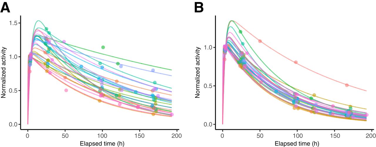
Figure 2 shows example time–activity data used to construct the data-driven models and the corresponding biexponential fits used to derive the reference TIA. The Teff, corresponding to the slowest component of the biexponential fit, had a median (±SD) value of 89.5 ± 35.5 h (range, 47.9–249.1 h) for tumors, 51.7 ± 13.4 h (range, 41.6–108.2 h) for left kidneys, 50.3 ± 14.4 h (range, 40.7–113.6 h) for right kidneys, and 51.2 ± 13.7 h (range, 40.7–113.6 h) for kidneys (Supplemental Fig. 1). These results agree well with reported values from other groups for similar cohorts (3,15–17), and the median values were used as Teff,p for the Madsen method in the current study. Only 2 of 54 kidneys had a Teff greater than 80 h and corresponded to the patient with the lowest eGFR in our cohort (Supplemental Table 1). Only 4 of 100 tumors (from 2 patients) had unusually high Teff (>150 h); however, in these cases, the investigation of clinical factors did not identify the reasons for the observed kinetics.

Example time–activity data and biexponential fits shown for select tumor, 1 tumor from each patient (A), and all left kidneys, corresponding to 27 patients (B). Curves are normalized to 4 h after therapy.
Prediction Model Analysis: Patient Data
Model 1
We found that the estimated curve from the GAM for model 1 (consisting of multiple basis functions) could be accurately reproduced by a simpler cubic function (Supplemental Fig. 2). To facilitate future implementation, we used the simpler cubic curve; explicit formulas are presented in Table 1.
Prediction Equations for Data-Driven Models
In Figure 3, TIA/A(t) is plotted as a function of time, with the function g(t) corresponding to the methods of Hänscheid, Madsen, and model 1. The function fits the data best in TP3 for kidneys and TP3 and TP4 for tumors. At other TPs, although g(t) corresponding to the Madsen method and model 1 fits the data reasonably well, this is not the case for the Hänscheid method. The GAM method makes the tradeoff between smoothness and accuracy of its prediction curve and possesses the desirable statistical property of being a consistent estimator.

Estimated g(t) curves with patient data as function of time for different STP methods for individual tumors (A) and kidneys (B).
Model 2
The LOOCV results when each of the biomarkers was included as auxiliary data in model 2 were compared with LOOCV results for model 1, for which auxiliary data were not used (Supplemental Table 2). On the basis of LOOCV, at TP1, the tumor volume was selected as a predictor of tumor TIA, and eGFR was selected as a predictor of kidney TIA over other biomarkers. At the other TPs, none of the considered biomarkers led to model enhancement. Using the same GAM method for estimating the potentially nonlinear effect of biomarkers, we selected a piecewise linear function of tumor volume for the tumor and linear functions of eGFR for kidneys (Table 1). Unlike at the other TPs, time is not a significant predictor at TP1 and thus does not appear in the corresponding prediction model. We presume this is due to the narrow range of time points included in TP1 (3–5 h).
STP Model Performance Comparison: Patient Results
Table 2 compares the performance of the different STP methods for TIA estimation. SDs are also shown to measure the patient variability. At TP3, all 4 methods performed very well for both tumors and kidneys: all had an MAE of less than 7% (SD < 10%), and more than 93% of tumors and kidneys had an absolute error of less than 20%. For tumors, all methods performed very well at TP4, with an MAE of less than 9%. At other TPs, the MAE for the Hänscheid method was substantially higher, whereas the Madsen method and data-driven methods performed reasonably well for both kidneys (MAE < 17%, SD < 20%) and tumors (MAE < 31%, SD < 32%). Adding auxiliary data (eGFR for kidneys and volume for tumors) to our data-driven model enhanced the performance at TP1 to achieve an MAE of less than 12% for kidneys and less than 27% for tumors.
Performance of STP Models for TIA Estimation in Patient Data
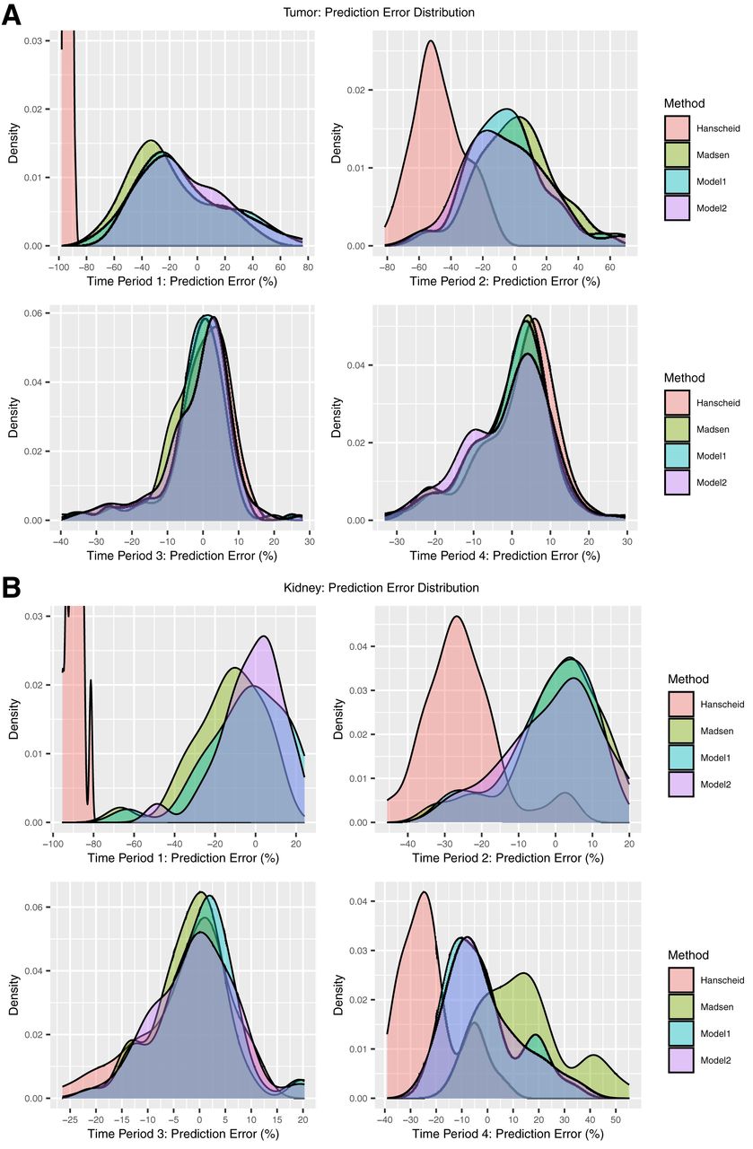
The density plots of the prediction error (Fig. 4) also demonstrated comparable performance at optimal TPs (TP3 and TP4 for tumors and TP3 for kidneys) for all methods. For the remaining nonoptimal TPs, the Hänscheid method resulted in substantial underestimation of the TIA, whereas the prediction error with the Madsen method and our data-driven methods was more centered at zero. At TP1 for tumors and kidneys, model 2 showed a modest improvement over the Madsen method and model 1.

Prediction error in TIA estimation for patient tumors (A) and kidneys (B) corresponding to different STP models. Negative error indicates underestimation of TIA by STP methods. Binned representation of model 2 prediction error is presented in Supplemental Figure 3. Period 1 = 3–5 h, period 2 = 23–51 h, period 3 = 72–126 h, period 4 = 144–193 h.
In addition to the relative errors shown in these figures and tables, a plot of predicted TIA from LOOCV versus reference TIA is included in Supplemental Figure 3.
STP Model Performance Comparison: Simulation Results
Supplemental Tables 3 and 4 and Supplemental Figure 4 show the results of testing on the simulated time–activity data. The results were consistent with the patient results: all 3 methods showed comparable performance at the optimal TPs (TP3 for kidneys and TP3 and TP4 for tumors), with an MAE of less than 12% for tumors and kidneys. At all other TPs, the Hänscheid method substantially underestimated the TIA, whereas the Madsen method and model 1 showed reasonable performance (MAE < 20% for kidneys and < 31% for tumors). Note that model 2 was not evaluated with simulation, given its reliance on patient biomarkers.
DISCUSSION
Taking advantage of existing multiple-time-point SPECT/CT data after [177Lu]Lu-DOTATATE PRRT for a cohort of patients, we tested the performance of TIA estimation with STP imaging, developing novel, data-driven methods. We demonstrated, for the first time, to our knowledge, the proof of concept of incorporating other standard clinical factors and biomarkers beyond the single activity measurement alone to potentially enhance the STP model performance. The prediction equations (Table 1) are valid for similar patients imaged after [177Lu]Lu-DOTATATE PRRT and generalizable for different acquisition or processing protocols as long as the TIA/A(t) ratio remains constant across the time points. For example, if on a different system the activity is always overestimated by 10% compared with our values because of a different calibration procedure, the TIA will also be overestimated by 10% and our prediction model remains valid.
Our results show that the optimal TP for the single measurement is in the range of 72–126 h after administration, an interval during which all methods evaluated performed very well, with an MAE of less than 7% for both kidneys and tumors. This is consistent with previous reports for [177Lu]Lu-DOTATATE PRRT (3–5,17), including the study by Hänscheid et al., which accordingly recommended a 96-h time point. However, practical considerations may lead to imaging of patients at other TPs. At these nonoptimal TPs, the Madsen method and our data-driven models provide reasonable prediction accuracy that is superior to that of the Hänscheid method (Fig. 4). At the earliest TP, which is likely the most convenient as it does not require a return visit to the clinic, adding eGFR and tumor volume into the data-driven models for kidneys and tumors, respectively, enhances STP prediction (model 2 MAE of 11.8% for kidneys and 27.1% for tumors; Table 2). It is worth noting that, with model 2, 83% of kidneys and 40% of tumors have an absolute error of less than 20%, with only 2 of 54 kidneys (both corresponding to the same patient) having an absolute error of more than 31% (Supplemental Fig. 5).
In addition to the methods of Madsen and Hänscheid, there are other recently reported methods for STP estimation by our group (18) and others (19,20). Devasia et al. (18) assumed biexponential kinetics and used a mixed-effect model to estimate the unknown fit parameters. Then a new patient’s STP measurement was combined with the assumed biexponential and the estimated parameters to make the TIA prediction. This approach does not involve a time-varying parameter and, as with the Hänscheid and Madsen methods, relies on the assumption of exponential kinetics across all time. Our present results suggest that exponential kinetics may not be accurate at the first TP because, in model 2, time is not a significant predictor of TIA, whereas tumor volume and eGFR are significant predictors (Table 1). Thus, a model whose parameters are data-driven and time-varying may be preferred. The method of Jackson et al. (19) can also be classified as a data-driven nonparametric STP model. They normalized existing time–activity curves to a single measurement time, making it possible to calculate a mean and range of TIA values that relate to the absorbed dose. Physiologically based pharmacokinetic models (20) use a system of differential equations to model the process of absorption and decay, on the basis of which the TIA can be calculated. However, this model has no explicit formula and requires mathematic software to make the predictions.
The advantages of data-driven models over physics-driven models mainly result from their property of local estimation (e.g., GAM (8) and local regression (21)), which means the prediction for an individual is based on patients in a localized subset who share similar features. Such models do not require the same global assumptions of physics-driven models and are therefore more flexible. As a result, the predictions are optimal across time points and robust to model misspecification. However, the local estimation property also has disadvantages. When the underlying model is correctly specified (e.g., if the time–activity data behave exponentially and the Teff is the same for all patients), data-driven models will be less efficient than parametric models such as Madsen method. This shortcoming is common to nonparametric models and is the result of the inherent trade-off between bias and variance (21). Although GAMs often use complex formulas for prediction, we were able to identify a much simpler model (Table 1) based on the fitted GAM (Supplemental Fig. 2)
The inclusion of biomarkers showed a moderate improvement in performance of the data-driven STP approach at TP1. Enhancement of the model for tumors with the inclusion of volume may be due to the kinetic differences between small and large tumors due to variations in tumor biology and microenvironment, which provide additional data not explained by the magnitude of SPECT uptake. The model for kidneys was enhanced by the inclusion of eGFR; this is unsurprising given that eGFR quantifies kidney function and directly influences the rate of activity uptake and clearance, providing additional kinetic information that is not available from SPECT uptake alone. Furthermore, eGFR has previously been demonstrated to predict kidney dosimetry in [177Lu]Lu-DOTATATE therapy (11). Notably, uptake on baseline [68Ga]Ga-DOTATATE PET/CT did not enhance the model performance for either tumors or kidneys (Supplemental Table 2) and thus was not included in the final model.
The level of accuracy that is needed to make dosimetry relevant to radiopharmaceutical therapy clinical practice depends on the application, that is, whether the role of dosimetry is in verifying treatment, in building models of absorbed dose versus outcome, or in planning and modifying treatment. For individualized planning, accuracy requirements for therapies delivered over several cycles—with absorbed dose estimates performed between cycles—are less stringent than for therapies delivered over 1 or 2 cycles. Regardless of the application, before STP estimates are used for clinical decision making, the variability in accuracy should be considered. The prediction error–density plots of Figure 4 and Supplemental Figure 4 indicate that, in general, the errors are negatively skewed for all STP methods, including at the optimal TP. This was previously reported for [177Lu]Lu-DOTATATE in both a theoretic study (22) and a clinical study with 777 kidneys (17), evaluating the methods of Hänscheid and Madsen. The negatively skewed error corresponds to an underestimation of TIA and, consequently, absorbed dose; hence, caution should be exercised when these methods are used for kidney dosimetry-guided treatment modification in individual patients. When dosimetry is performed with STP imaging instead of multiple-time-point imaging, a wider safety margin can be used for the kidney-absorbed dose limit, for example, based on reported prediction error distribution (Fig. 4) in studies such as ours. Protocols can also be designed to switch to multiple-time-point imaging in the next cycle as a cautionary measure only for those patients whose STP-estimated kidney-absorbed dose in the previous cycle is above a limit predetermined on the basis of the predicted error distribution for the specific STP model.
To mitigate the limitations due to the small size of our clinical dataset, we used bootstrap methods to generate simulated data with a larger sample size. The simulation also allowed us to compare methods under different noise conditions and with the true TIA available. However, the simulation study could not include data-driven model 2 because of the need for biomarker information. Furthermore, the limited sample size confined our biomarker selection for model 2 to a more conservative approach to avoid overfitting; hence, only univariable models were considered. Although we used internal validation (cross validation), external independent validation of our data-driven models, which are specific to [177Lu]Lu-DOTATATE, should be performed before clinical implementation.
CONCLUSION
The STP methods for TIA estimation in dosimetry that were proposed in the current study performed equally as well as previous physics-based methods (MAE < 7%) for both kidneys and tumors at the optimal TP of days 3–5 after [177Lu]Lu-DOTATATE PRRT. At other TPs (days 0–2 and days 6–8), our data-driven models and the Madsen model performed reasonably well, especially for kidney TIA, where the MAE was less than 17%. Adding auxiliary data to the single activity measurement enhanced the performance of the data-driven model for kidneys at TP1, where an MAE of less than 12% (SD < 15%) was achieved with the inclusion of eGFR.
DISCLOSURE
This work was supported by grants R01CA240706 and P30CA046592 from the National Cancer Institute. No other potential conflict of interest relevant to this article was reported.
KEY POINTS
QUESTION: How accurate is the STP-imaging–based TIA estimation for dosimetry in [177Lu]Lu-DOTATATE PRRT when imaging is performed at a nonoptimal time point?
PERTINENT FINDINGS: Although the optimal time point is from day 3 to day 5, the Madsen and the proposed data-driven STP methods provide a reasonable estimate (MAE < 17% for kidneys and < 31% for tumors) for time points from day 0 to day 8. At day 0, the model incorporating baseline biomarkers outperforms other methods, achieving an MAE of less than 12% for kidneys.
IMPLICATIONS FOR PATIENT CARE: STP methods that are less sensitive to time-point selection and perform well even with early imaging (day of therapy) provide flexibility to the patient and clinic, enhancing the feasibility of radiopharmaceutical therapy dosimetry in clinical practice.
Footnotes
Published online Jul. 27, 2023.
- © 2023 by the Society of Nuclear Medicine and Molecular Imaging.
REFERENCES
- Received for publication December 22, 2022.
- Revision received April 27, 2023.


