


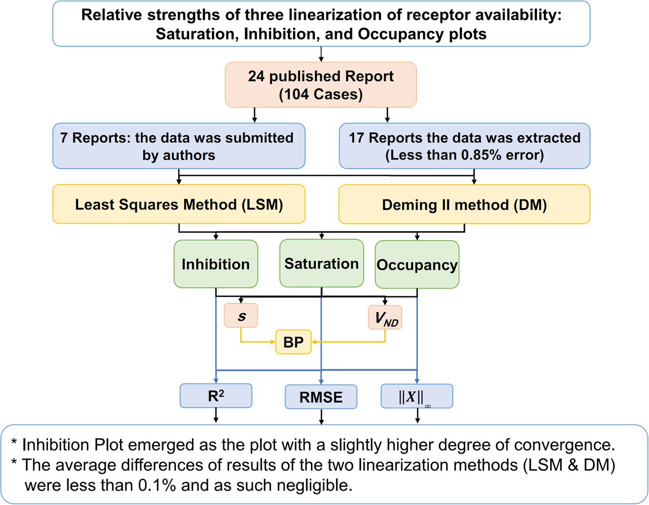
Visual Abstract

Abstract
We derived three widely used linearizations from the definition of receptor availability in molecular imaging with positron emission tomography (PET). The purpose of the present research was to determine the convergence of the results of the 3 methods in terms of 3 parameters—occupancy (s), distribution volume of the nondisplaceable reference binding compartment (VND), and nondisplaceable reference binding potential (BPND) of the radioligand—in the absence of a gold standard. We tested 104 cases culled from the literature and calculated the goodness of fit of the least-squares and Deming II methods of linear regression when applied to the determination of s, VND, and BPND using the goodness-of-fit parameters R2, coefficient of variation (root-mean-square error [RMSE]), and the infinity norm (‖X‖∞) with both regression methods. We observed superior convergence among the values of s, VND, and BPND for the inhibition and occupancy plots. The inhibition plot emerged as the plot with a slightly higher degree of convergence (based on R2, RMSE, and ‖X‖∞ value). With two regression methods (the least-squares method [LSM] and the Deming II [DM] method), the estimated values of s, VND, and BPND generally converged. The inhibition and occupancy plots yielded the best fits to the data, according to the goodness-of-fit parameters, due primarily to absence of commingling of the dependent and independent variables tested with the saturation (original Lassen) plot. In the presence of noise, the inhibition and occupancy plots yielded higher convergences.
PET is a major tool of biomedical research, with clinical applications that yield images of the distribution of systemically administered positron-emitting radionuclides in tomographic sections of the bodies of human subjects and experimental animals (1,2). Positrons are positively charged anti-electrons emitted from the nuclei of short-lived isotopes typically produced in a cyclotron. Users of this technique image the high-energy (511 keV) annihilation photons that result from the interaction of a positron with electrons in the tissue. PET images are reconstructed by means of computed tomography of the source of radioactivity, after injection of radiopharmaceuticals according to the principles of nuclear medicine (3). The imaging of neuroreceptors with radioactive ligands by PET applied to living mammalian brains makes it possible to determine receptor density and affinity by appropriate mathematic models (4).
Neuroreceptor studies of brain in vivo using PET require comparisons of so-called binding potentials of radiopharmaceutical receptor ligands at more or less inhibited receptor states to obtain estimates of receptor density and affinity (5). Naganawa et al. (6) proposed methods that reduce bias and variability, and the best use of these approaches is realized by improving the accuracy of data covariance matrices.
The quantitative determination of binding potentials uses a fundamental equation of receptor availability to obtain separate estimates of radioligand volumes of distribution of a specific radioligand (5,7–10). Application of any one of the three linearizations presented here is the first step toward determining binding potentials (or receptor availabilities), the foundation of the receptor-binding analysis. For situations in which a proper reference region with no specific binding of the ligand is not known to exist, or is known not to exist, three linearized versions of a receptor availability equation were derived to estimate the magnitude of the volume of distribution of nondisplaceable ligand (VND) by linear regression. The three different plots emerged when the equation of receptor availability was linearized differently by Lassen et al., Gjedde and Wong, and Cunningham et al. (11–13). Here, the three different plots are referred to as the Saturation, Inhibition, and Occupancy plots, to avoid the uncertain naming of the plots associated with the presentation of the Occupancy plot solution (12), referred to by some authors as the Lassen plot rather than the plot that Lassen et al. (11) actually used and reported. The Occupancy and Saturation plots commingle the dependent and independent variables by calculating the difference between the volume estimates for baseline and inhibition states, unlike the Inhibition plot, which simply plots the apparent total volume of distribution of the radioligand (VT, also known as the partition volume or partition coefficient of the ligand) at inhibition (VT(i), ordinate) against the values at baseline (VT(b), abscissa).
The aim of the present research was to determine the accuracy and precision of these three widely used linearizations of receptor availability (Saturation, Inhibition, and Occupancy plots) from experimental data. We compared 104 cases culled from the literature, with the accuracy of each plot being evaluated by the least-squares and Deming II methods of linear regression.
MATERIALS AND METHODS
The quantitative determination of binding potentials uses a fundamental equation of receptor availability to obtain separate estimates of radioligand volumes of distributions for a specific radioligand (5,7–10):
 (1)
where Equation 1 is the formulation of the relative or fractional receptor availability in terms of the relevant volumes of distribution. Here, s represents the occupancy and VT(i) is the apparent total volume of distribution of the sum of the specifically bound and the nonspecifically dissolved ligand molecules occupying the receptor, whereas VND refers to the distribution volume of the tracer in a nonbinding compartment, also known as the partition volume or partition coefficient of the ligand. VT(b) refers to the apparent total volume of distribution of the radioligand in a baseline state where the receptor is not occupied by a specific inhibitor.
(1)
where Equation 1 is the formulation of the relative or fractional receptor availability in terms of the relevant volumes of distribution. Here, s represents the occupancy and VT(i) is the apparent total volume of distribution of the sum of the specifically bound and the nonspecifically dissolved ligand molecules occupying the receptor, whereas VND refers to the distribution volume of the tracer in a nonbinding compartment, also known as the partition volume or partition coefficient of the ligand. VT(b) refers to the apparent total volume of distribution of the radioligand in a baseline state where the receptor is not occupied by a specific inhibitor.
Application of any one of the three linearizations presented here is the first step toward determining binding potentials (or receptor availabilities), the foundation of the receptor-binding analysis. The non-displaceable reference binding potential (BPND) enters into the particular Eadie–Hofstee version of the linearized Michaelis–Menten equation that yields both the maximum binding (Bmax) and the affinity constant (Michaelis half-saturation quantity or mass), KD, of the receptors,
 (2)
where B is the quantity of bound ligand. The binding potential is defined as the ratio of the volumes of distribution of specifically bound (displaceable) and non-specifically bound (non-displaceable) ligand quantities (14,15). To determine the binding potential of a radioligand, the volumes of distribution are entered into the relationship that defines the binding potential (2,5,16):
(2)
where B is the quantity of bound ligand. The binding potential is defined as the ratio of the volumes of distribution of specifically bound (displaceable) and non-specifically bound (non-displaceable) ligand quantities (14,15). To determine the binding potential of a radioligand, the volumes of distribution are entered into the relationship that defines the binding potential (2,5,16):
 (3)
which is applicable both to the receptor binding baseline and to multiple degrees of receptor blockade, provided the VND estimate is unaffected by the blockade. To calculate binding potentials, it is necessary to know the distribution of unbound ligand in a region of no binding, but a suitable reference region often does not exist or is not known to exist.
(3)
which is applicable both to the receptor binding baseline and to multiple degrees of receptor blockade, provided the VND estimate is unaffected by the blockade. To calculate binding potentials, it is necessary to know the distribution of unbound ligand in a region of no binding, but a suitable reference region often does not exist or is not known to exist.
The three linearizations evaluated here served to determine a reference volume of distribution of radioligands when no reference region (i.e., a region with absence of specific binding) is known to exist in the brain. From the volumes of distribution of the radioligand in the absence of displaceable binding (VND), we used the three different linearizations to obtain binding potentials for radioligands used in published studies.
Saturation Plot
As a novel steady-state approach to determining the binding potentials of tracers with an unknown reference volume of distribution, in 1995, Lassen et al. (11) proposed to compare two levels of receptor occupancy, one essentially at zero for the labeled tracer itself and the other in the midrange of occupancy by addition of unlabeled ligand. The concentration of the unlabeled ligand in brain water would be zero in the tracer-alone study and would have a constant value in the inhibition studies. To obtain the volume of nonspecific binding, Lassen et al. (11) linearized Equation 1 in the form of the plot we here call the Saturation plot. The plot yields the estimate of VND by plotting the baseline volume of distribution (VT(b)) as a function of the difference between the baseline and inhibition volumes of distribution ( ) as shown in Figure 1A,
 (4)
where the estimate of VND is the ordinate intercept of the linear regression, and the estimate of the ratio 1/s is the slope of the regression.
(4)
where the estimate of VND is the ordinate intercept of the linear regression, and the estimate of the ratio 1/s is the slope of the regression.

Three linearization plots ([A] Saturation, [B] Inhibition, [C] Occupancy) of data from Horti et al. (17) (inhibition dose 0.5 mg).
Inhibition Plot
Certain receptor ligands tend altogether to lack a reference brain region of no specific binding, from which it is therefore not possible to assess nonspecific binding for the purpose of calculating the binding potential in regions of specific binding. Realizing that the uncertain choice of a reference volume of distribution for the ligand can lead to an erroneous estimation of the occupancy, in 2000, Gjedde and Wong (12) proposed to linearize Equation 1 to obtain the form of the Inhibition plot. The plot estimates VND by relating VT(i) to VT(b) by linear regression, as shown in Figure 1B,
 (5)
where the estimate of VND is the intercept of the linear regression line with the line of identity.
(5)
where the estimate of VND is the intercept of the linear regression line with the line of identity.
Occupancy Plot
In 2010, Cunningham et al. (13) inverted the axes of the Saturation plot and showed that the graphical analysis of the inverted relationship at each of the different doses of unlabeled ligand provided a means to determine drug occupancies. The inversion of the axes of the Saturation plot was presented as the Occupancy plot, a term we adopt here to avoid the lack of specificity of the term Lassen plot. The linearization known as the Occupancy plot treats the differences in the volumes of distribution between the baseline and challenge conditions,  , as a function of the baseline volume of distribution, as shown in Figure 1C,
 (6)
where VND is the abscissa intercept. It is evident from the derivations that the Saturation and Occupancy plots have mutually inverted axes.
(6)
where VND is the abscissa intercept. It is evident from the derivations that the Saturation and Occupancy plots have mutually inverted axes.
Source of Published Data
To use any one of the three linearizations, at least two consecutive PET recordings with two different levels of receptor occupancy are required. For the Inhibition plot, unlike the Saturation and Occupancy plots, the dependent (VT(i)) and independent (VT(b)) variables are not commingled. The estimates of the fractional receptor availability (1 − s) and VND are then obtained directly from the volumes of distribution. As the three linearizations are derived from the same original relative receptor availability formulation (Eq. 1), they must all meet the requirements that there are different brain regions with different receptor densities (maximum binding) that remain unchanged in the challenge condition and that the values of receptor affinity (Michaelis half-saturation concentration) and VND are the same for all relevant regions and remain the same for all challenges.
To assess the advantages and disadvantages of each of the three linearizations, the following names were searched in the PubMed and Scopus databases: “Lassen plot,” “Saturation plot,” “Gjedde plot,” “Inhibition plot,” “Cunningham plot,” and “Occupancy plot.” In the initial search, 60 published reports were found. The original datasets were not available for 36 of the identified studies.
Linear Regressions of Published Data
We analyzed the 24 remaining published reports, which consisted of 104 sets of data. In 7 cases, the authors submitted data (8,17–22), and for the remaining 17 reports, we extracted the data from published graphs with GetData Graph Digitizer digitization software (11,13,23–37). The characterization of the data in terms of species, sex, age, drug, dose, and other identifiers is presented in Table 1. We used two linear regression methods, LSM and DM, to obtain parameter estimates, as implemented in MATLAB (MathWorks). Using slope and intercept estimates, we determined s and VND and evaluated the accuracy.
Categorization of Data
LSM is a standard approach in regression analysis, with its most important application being in data fitting. The best fit of LSM minimizes the sum of squared residuals, which are the differences between an observed value and the value fitted by the model. In LSM, 2 variables (x,y) are obtained by regression of y on x, where x is assumed to represent independent-variable values obtained without error (38). DM regression is an errors-in-variables model that yields the line of best fit for a 2-dimensional dataset. It differs from LSM by the assumption of errors in both independent and dependent variables that allow for any number of predictors and a more complicated error structure. In DM, observations are subject to additive random variations of both x and y (39,40).
To test the goodness of fit of the linear regressions, we calculated the coefficient of determination (R2), coefficient of variation (root-mean-square error [RMSE]), and infinity norm (‖X‖∞). The R2 estimate is a commonly used indicator of the goodness of fit that is applicable only to LSM, as in other applications it may result in negative values or values greater than unity. In contrast, RMSE is applicable to all linear regressions. For n sets of (xi; yi) data, the RMSE, R2, and ‖X‖∞ measures can be expressed according to Rawlings et al. (38):
 (7)
(7)
 (8)
where n is the number of observations, and
(8)
where n is the number of observations, and
 (9)
where fi is the predicted value of y at xi, SStot is the total sum of squares or the variance of the data,
(9)
where fi is the predicted value of y at xi, SStot is the total sum of squares or the variance of the data,
 (10)
SSres is sum of squares of residuals,
(10)
SSres is sum of squares of residuals,
 (11)
and
(11)
and  is the mean of yi,
 (12)
The closer the value of R2 is to unity, the better the fit is to the linearization. The closer the RMSE and ‖X‖∞ values are to zero, the better the fit of the linearization is held to be (38,41).
(12)
The closer the value of R2 is to unity, the better the fit is to the linearization. The closer the RMSE and ‖X‖∞ values are to zero, the better the fit of the linearization is held to be (38,41).
Calculation and Evaluation of Binding Potentials
We compared binding potential estimates (BPND) for the baseline (base BPND) and inhibition (challenge BPND) conditions according to Equation 3. In total, we compared 104 times 12, or 1,248, sets of BPND estimates according, first, to the equation for the percentage differences in the LSM and DM results for each of the 3 linearizations, exemplified here for the inhibition plot as
 (13)
and, second, according to the equation for the percentage differences in the three linearizations of each of the two regression methods, exemplified here for the comparison of LSM and DM results for the Inhibition and Occupancy plots,
(13)
and, second, according to the equation for the percentage differences in the three linearizations of each of the two regression methods, exemplified here for the comparison of LSM and DM results for the Inhibition and Occupancy plots,
 (14)
and
(14)
and
 (15)
(15)
Goodness of Fit
We considered sets of data (VT(b), VT(i)) directly measured in relevant studies. Because of sources of error, which include surgery, environment, and device errors, we predicted differences to exist between the theoretic but unknown value of a parameter and the measured value (42). We expressed the theoretic value of a parameter as (VT(b), VT(i)),
 (16)
and
(16)
and
 (17)
where
(17)
where  and
and  are the differences between real and measured values of VT(b) and VT(i), respectively. We expressed the real value of the differences between baseline and inhibition volumes of distribution as
  ,
,
 which after substitution yielded,
 or
or
 which yielded,
 (18)
where e3 refers to the difference between the real and measured values of ΔVT.
(18)
where e3 refers to the difference between the real and measured values of ΔVT.
Source of Convergence
In this research, we defined the closeness of the fitted model to the data as convergence. For the set of (xi; yi), regardless of method, the linearization has the form,
 (19)
with the real values in the equation expressed as,
(19)
with the real values in the equation expressed as,
 (20)
where (a,b) are the estimated values of slope and ordinate intercept and (a*,b*) are the real values of slope and ordinate intercept. As discussed, the measurement error of (xi; yi) yields a difference between real and estimated values of slope and ordinate intercept as
(20)
where (a,b) are the estimated values of slope and ordinate intercept and (a*,b*) are the real values of slope and ordinate intercept. As discussed, the measurement error of (xi; yi) yields a difference between real and estimated values of slope and ordinate intercept as
 (21)
and
(21)
and
 (22)
where
(22)
where  is the error between real and estimated values of slope and ordinate intercept. By substituting Equations 20 and 21 in the 3 original equations (Eqs. 4–6), we calculated the differences between real and estimated values of s and VND. Here, occupancy and VND are the estimated values, and s* and VND* are the real (unknown) values. The differences between the real and estimated values of s and VND are listed in Table 2.
Differences Between Real and Estimated Values of s and VND of Inhibition, Occupancy, and Saturation Plots
RESULTS
Digitization Accuracy
We compared the linearizations of data obtained from the authors directly or by digitization of published graphs. With the submitted data available for comparison, we showed the mean error of digitization to be less than 0.85%, confirming the accuracy of the digitization. Here, we present the results from the analysis of the digitized values of VT(b) and ΔVT from the report of Horti et al. (17), used to obtain the VT(i) values for the 0.5-mg receptor inhibitor challenge. With the Inhibition, Saturation, and Occupancy linearizations for the LSM and DM regressions, we obtained the parameter values from the linear regressions of the data presented in Figure 1, with the resulting regressions and estimates of s and VND being presented in Figure 2. For the Saturation plot, we used ΔVT as the independent variable (x) and VT(b) as the dependent variable (y), whereas for the Occupancy plot, we used ΔVT as the dependent variable (y) and VT(b) as the independent variable (x).

Average values of measures of goodness of fit of the Inhibition, Saturation, and Occupancy plots.
Plot Analysis
Using the linearization goodness-of-fit parameters R2, RMSE, and ‖X‖∞, the comparisons yielded the results listed in Table 3 and Figure 2. The mean value of R2 (for the 104 samples) for the Inhibition plot was slightly closer to unity, identifying the Inhibition plot as the plot with slightly greater fit to the experimental data. In addition, the mean values of RMSE and ‖X‖∞ for the Inhibition plot were closest to zero, again as the most accurate of the three plots. In 87 of the 104 cases, the Inhibition plot yielded the lowest RMSE and ‖X‖∞ values, implying that the inhibition plot had superior accuracy in the 87 cases.
Average Precision of Regressions of Inhibition, Occupancy, and Saturation Plots
The effects of the regression method (LSM or DM) on the estimated values of s, VND, and BPND are shown in Figure 3. The estimates of s, VND, and BPND for the two regression methods (LSM and DM) generally converged. The average deviation was less than 0.1% for s and VND and was less than 3% for BPND. We also compared the effects of choice of method on the estimated values of s, VND, and BPND. The deviations of s, VND, and BPND for the three plots (Inhibition, Saturation, and Occupancy) are shown in Figure 3. From the figure, we conclude that the results of the Inhibition and Occupancy plots normally converged for both LSM and DM. The average difference of the inhibition and occupancy plot results was less than 2%. In contrast, we generally found considerable differences between the results of the Saturation plot and the results of the Inhibition and Occupancy plots. The average difference shown in Figure 3 is close to 40%. Bland–Altman graphs for the binding potentials determined with 0.5-mg receptor inhibitor blockade by Horti et al. (17) are shown in Supplemental Figure 1 (supplemental materials are available at http://jnm.snmjournals.org).

Differences of s, VND, and BPND among Inhibition, Saturation, and Occupancy plots. (A) s and VND LSM vs. Deming II. (B) BPND LSM vs. Deming II. (C) VND LSM and Deming II in different plots. (D) BPND Base LSM and Deming II in different plots. (E) s LSM and Deming II in different plots. (F) BPND Challenge LSM and Deming II in different plots.
Analysis of Noise Simulation
To investigate the effect of noise on the convergence of the results of different plots, two sets of theoretic data (data without noise) were created on the basis of the Horti et al. (17) data at two levels of inhibition (0.5- and 5-mg inhibitor administration). We considered five sets of data and calculated the values of s and of VND using the three plots and two different linearizations (data without noise; data with noise of K = 0.1, K = 0.2, K = 0.5, where K is the chosen SD). The results of the linearizations are listed in Supplemental Table 1 and Supplemental Figure 2. As shown in Supplemental Figure 3, for the data without noise, all three plots and two linearizations yield identical results. For the convergence of the three plots, it is evident that the RMSE of the data without noise for all three plots is approximately zero (10−9). However, as is shown in Supplemental Figure 4, in the presence of noise, the inhibition and occupancy plots yielded a lower RMSE, consistent with greater convergence.
DISCUSSION
In the present examination of the plots of competition, we linearized the formulation of the fractional receptor availability (Eq. 1) into three equations underlying the different regressions, which we refer to as the Saturation, Inhibition, and Occupancy plots. The purpose of all three linearizations is to estimate the reference volume of distribution, VND, required to calculate the binding potential of a radioligand. We undertook the comparisons because the extent to which the results of the three plots converge or diverge is unknown. We culled 104 cases on the basis of one or more of the plots, and we tested the results of the three plots linearized by LSM and DM regressions.
As shown in Table 3, for both s and VND, the differences between estimated and real values are of the same order of magnitude for the Inhibition and Occupancy plots but are much greater for the Saturation plot. For this reason, the average deviation of the calculated values of s and VND for the Inhibition and Occupancy plots was less than 0.1%, and the results generally converged. In contrast, there was more than a 35% difference between the results of the Saturation plots and the results of the Inhibition and Occupancy plots. In Equations 16–18, e1, e2, and e3 are the error values resulting from the divergence of individual plots. The parameter e3 may be smaller than e1 and e2 but frequently is not. As e1 and e2 do not adopt exclusively positive or negative values, errors can be superimposed. For this reason, the use of ΔVT differences may result in higher levels of error and reductions of goodness of fit. Among the three methods, the Inhibition plot avoided the use of the commingled variable ΔVT. As expressed by the three indicators R2, RMSE, and ‖X‖∞, the Inhibition plot was shown to yield slightly greater fit for both LSM and DM. The noise analysis showed that the Inhibition and Occupancy plots yielded higher convergence in the presence of noise.
CONCLUSION
On the basis of all three goodness-of-fit parameters (R2, RMSE, and ‖X‖∞), and using both regression methods (LSM and DM), the Inhibition and Occupancy plots emerged as the plots with a superior degree of convergence. We judge this to be in part because of the absence of commingling of the original dependent and independent variables of the Saturation (original Lassen) plot. Concerning the effect of regression method (LSM and DM) on the estimated values of s, VND, and BPND, we observed that the average differences in the results of the Inhibition and Occupancy plot linearizations were less than 0.1% and, as such, negligible. In contrast, we noted more than a 35% difference in the results of the Saturation plot comparisons—a difference that we explain by the violation of the negligible variability rule for independent variables. The noise analysis showed that the three plots resulted in the same parameter estimates in the absence of noise. However, in the presence of noise, the Inhibition and Occupancy plots yielded higher and close degrees of convergence.
DISCLOSURE
This study was supported by Parkinsonforeningen, Lundbeckfonden (R77-A6970), and the Danish Agency for Science and Higher Education. No other potential conflict of interest relevant to this article was reported.
KEY POINTS
QUESTION: Which of the three linearizations (Inhibition, Saturation, and Occupancy) had superior convergence with the experimental results?
PERTINENT FINDINGS: Superior convergences among the values of s, VND, and BPND were observed for the Inhibition and Occupancy plots. On the basis of the goodness-of-fit parameters (R2, RMSE, and ‖X‖∞) and with both regression methods (LSM and DM), the Inhibition plot emerged as the plot with the slightly higher degree of convergence.
IMPLICATIONS FOR PATIENT CARE: The correct use of the Occupancy and Inhibition plots allows brain-imaging specialists to advise on the optimal dose of target engagement of neuroreceptor inhibitor drugs chosen to block the pathologic excess of neurotransmission.
Footnotes
Published online June 04, 2021.
- © 2022 by the Society of Nuclear Medicine and Molecular Imaging.
REFERENCES
- Received for publication December 15, 2020.
- Revision received April 23, 2021.
In this issue


Jump to section
Related Articles
Cited By...
- No citing articles found.