


Abstract
Scintillation camera images contain a large amount of Poisson noise. We have investigated whether noise can be removed in whole-body bone scans using convolutional neural networks (CNNs) trained with sets of noisy and noiseless images obtained by Monte Carlo simulation. Methods: Three CNNs were generated using 3 different sets of training images: simulated bone scan images, images of a cylindric phantom with hot and cold spots, and a mix of the first two. Each training set consisted of 40,000 noiseless and noisy image pairs. The CNNs were evaluated with simulated images of a cylindric phantom and simulated bone scan images. The mean squared error between filtered and true images was used as difference metric, and the coefficient of variation was used to estimate noise reduction. The CNNs were compared with gaussian and median filters. A clinical evaluation was performed in which the ability to detect metastases for CNN- and gaussian-filtered bone scans with half the number of counts was compared with standard bone scans. Results: The best CNN reduced the coefficient of variation by, on average, 92%, and the best standard filter reduced the coefficient of variation by 88%. The best CNN gave a mean squared error that was on average 68% and 20% better than the best standard filters, for the cylindric and bone scan images, respectively. The best CNNs for the cylindric phantom and bone scans were the dedicated CNNs. No significant differences in the ability to detect metastases were found between standard, CNN-, and gaussian-filtered bone scans. Conclusion: Noise can be removed efficiently regardless of noise level with little or no resolution loss. The CNN filter enables reducing the scanning time by half and still obtaining good accuracy for bone metastasis assessment.
Scintillation camera images are inherently noisy because of the specifics of the imaging process. Several filtering methods to remove noise exist, which range from simple convolution with small filter kernels to more complex filtering using wavelets or statistical methods (1–4). However, the trade-off for most types of denoising filters is resolution loss.
Convolutional neural networks (CNNs), a machine learning algorithm, have been shown to work well in denoising photographic images. These types of images generally contain only a small amount of noise, making it easy to generate sets of noisy and pristine photographic images to train a CNN. Scintillation camera images, however, suffer from a larger amount of Poisson noise. Thus, it is more challenging to acquire sets of noisy and pristine image sets for training purposes.
It is believed that machine learning will change radiology and nuclear medicine in the future (5). There have been recent publications on the use of machine learning algorithms for classification and segmentation purposes (6–10). CNNs have been used to obtain standard-dose CT and PET images from low-dose data (11,12) and to enhance images by determining scatter correction parameters (13) and CNN-augmented emission-based attenuation correction (14) in PET. Recently, Gong et al. used computer-simulated PET images to pretrain a denoising CNN and then fine-tuned the CNN with patient data (15). The same group has also implemented a CNN in the reconstruction process for PET data (16).
This study investigated whether noise can be removed from scintillation camera images using a CNN that has been trained with sets of noisy and noiseless images obtained by Monte Carlo simulation and whether the types of training images affect the results. If a CNN is to be used for any type of medical image enhancement, it is vital that no true information be removed or false information added to the images. The CNN should recreate only information that has been lost in the imaging process. The question is whether a single CNN can be trained and used on multiple types of images or whether specialized CNNs that are trained and used on only one type of images (e.g., bone scans) are needed.
The aim of this study was to generate different CNNs using different sets of training images and to evaluate the performance of the CNNs on simulated images of a cylindric phantom and simulated whole-body bone scan images. We compared the CNN-filtered images with images filtered with gaussian and median filters. As a proof of concept, we performed a pilot clinical evaluation in which bone scans with half the number of counts were filtered using the CNN and gaussian filter and then compared with standard bone scans for the diagnosis of bone metastases.
MATERIALS AND METHODS
Training Images
Noiseless whole-body bone scan images were generated with the Simind Monte Carlo program and the XCAT anthropomorphic phantom (17,18). Three different phantoms were used, and 60 different simulations were generated with random numbers and sizes of bone metastases ranging from 1 to more than 50. The method used to create and simulate phantoms with different tumor burdens was previously described (8). Both anterior and posterior views were simulated, and the simulations included all physically degenerative effects such as attenuation and scatter in the phantom, scatter in and penetration of the collimator, and depth-dependent resolution. The Simind program was set up to mimic a Siemens Symbia γ-camera using a 256 × 1,024 matrix with a pixel size of 2.21 mm and a 15% energy window centered over the 140-keV peak. Next, 10,000 noiseless training images were created by randomly extracting a 256 × 256 patch from either the anterior view or the posterior view of a simulated image, applying a random shearing operation on the patch (to generate images with various body shapes and sizes), and multiplying the patch by a random number so that the total number of counts in the corresponding whole-body image would range from 0.5 to 3 million counts (bone scan guidelines recommend at least 1.5 million counts (19)). The patches were then downsized to a matrix size of 128 × 128.
A second training set was created with the Simind Monte Carlo program using a simple cylindric phantom with a homogeneous activity distribution. Three phantoms with a length of 30 cm, a long axis of 15 cm, and short axes of 5, 10, or 15 cm were simulated with the same camera setup as for the bone simulation. Fifteen projections evenly sampled in an arc of 0°–90°, with the starting angle parallel to the short axis, were simulated for each phantom to create 45 different images in total. For each cylinder, 3 different simulations with small ellipsoids were performed in the same way with the ellipsoid in the middle of the cylinder.
Next, 10,000 noiseless training images were created by randomly selecting a projection from 1 of the 3 simulations. One or more hot spots or cold spots were then added at random places in the image of the cylinder by randomly choosing an image from the ellipsoid simulations, multiplying it by a random number, translating it in a random manner, and finally adding or subtracting it from the cylinder image. The cylinder images were then multiplied by a random number to mimic a range of intensity levels that are normally seen in nuclear medicine images. Finally, a random affine transformation was applied, which included translation, rotation, shearing, and scaling. Examples of the sets of noiseless and noisy images are displayed in Figure 1.

(Top row) Two examples from training batch with cylindric phantoms. (Bottom row) Two examples from training batch with bone scans. Images to left are noiseless, and images to right are noisy.
CNN
A denoising CNN (20) has shown good results in denoising ordinary color photographs, and hence, the same network structure was used in this work. This type of network has 3 parts. The first is a convolutional layer with 64 3 × 3 filters and a rectified linear unit activation. There are also 19 convolutional layers, which each have 64 filters with a size of 3 × 3, batch normalization, and rectified linear unit activation. Finally, a convolutional layer with a single 3 × 3 filter produces the output image.
The CNNs were trained using a quadratic loss function in MATLAB (MathWorks). Three different CNNs were evaluated: one using only bone scan images for training (further called bone CNN), a second using only cylinder images (cylinder CNN), and a third using a mix of images (mix CNN). Each CNN was trained using 10,000 different images. Four noisy patches per noiseless image were used for training, leading to a total of 40,000 training images. Random Poisson noise was added to the images corresponding to the intensity level of the images. Training was performed on an nVidia GeForce RTX 2080 TI graphics processing unit.
Evaluation
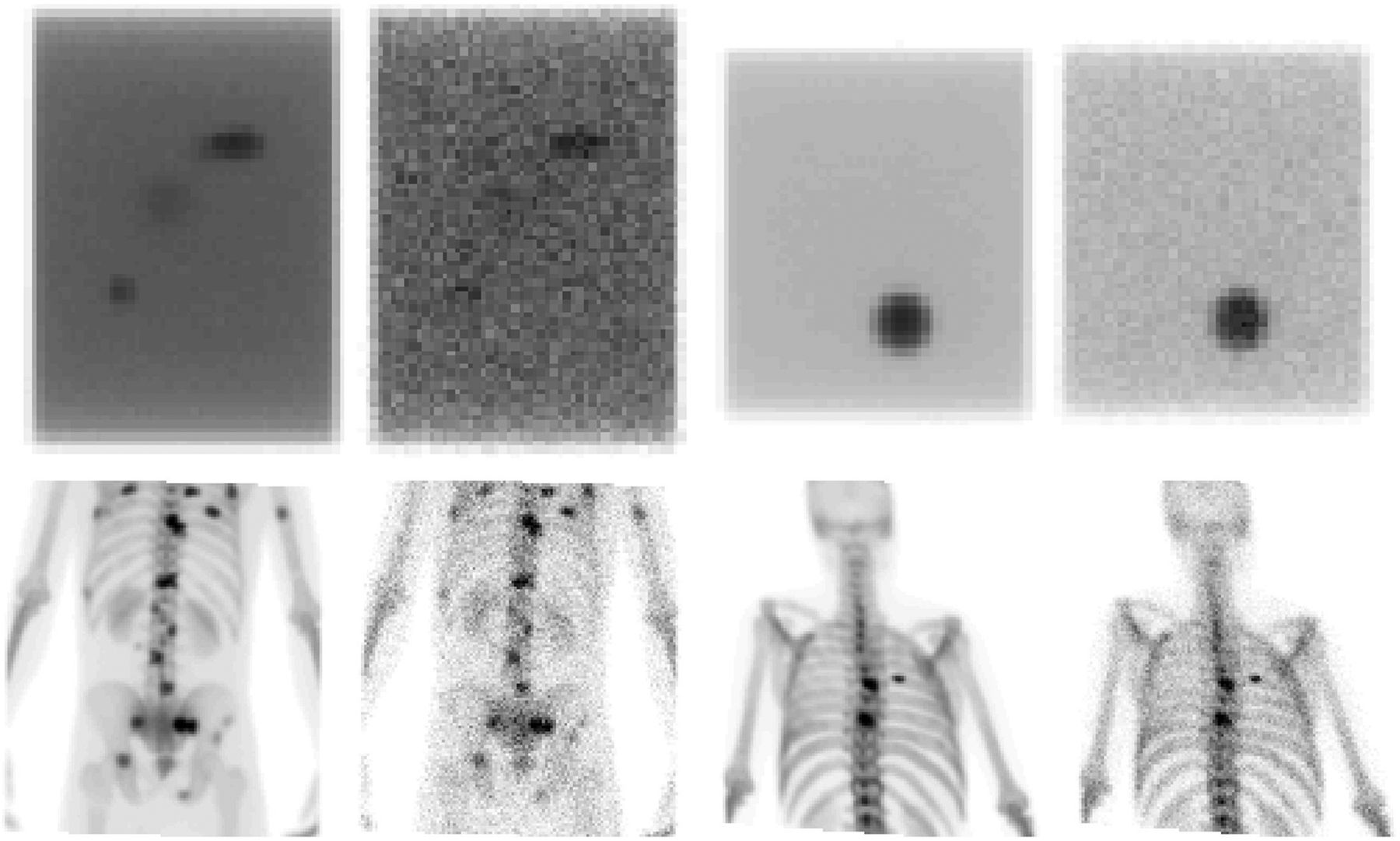
A simulation of a cylindric phantom was used, which consists of a 15-cm-high cylinder with a radius of 15 cm, with the camera placed perpendicular to the height direction of the cylinder. Several hot spheres with radii of 0.5, 0.6, 0.7, 0.8, 0.9, 1.0, 1.2, and 1.4 cm and 4 cold spheres with radii of 0.5, 1.0, 1.5, and 2.0 cm were placed in the middle of the cylinder in the height direction (Fig. 2). The activity ratio of hot spot to background was 10:1, which yields a maximum contrast of around 2.4 for the large hot spot, when accounting for attenuation and overlapping background activity. Ten images with a total number of counts ranging from 100,000 to 1 million were created, and 40 noise realizations per image were generated. All the noisy images were filtered with the different CNNs and with 6 different gaussian filters with full widths at half maximum of 3, 5, 7, 9, 11, and 13 mm, respectively. Four different median filters were also used with quadratic kernels of 9, 25, 49, and 81 pixels.

Simulated cylindric phantom. Images in top row have 1 million counts, and those in bottom row have 100,000 counts. From left to right: noisy image; images filtered with bone CNN, cylinder CNN, and mix CNN; and true image.
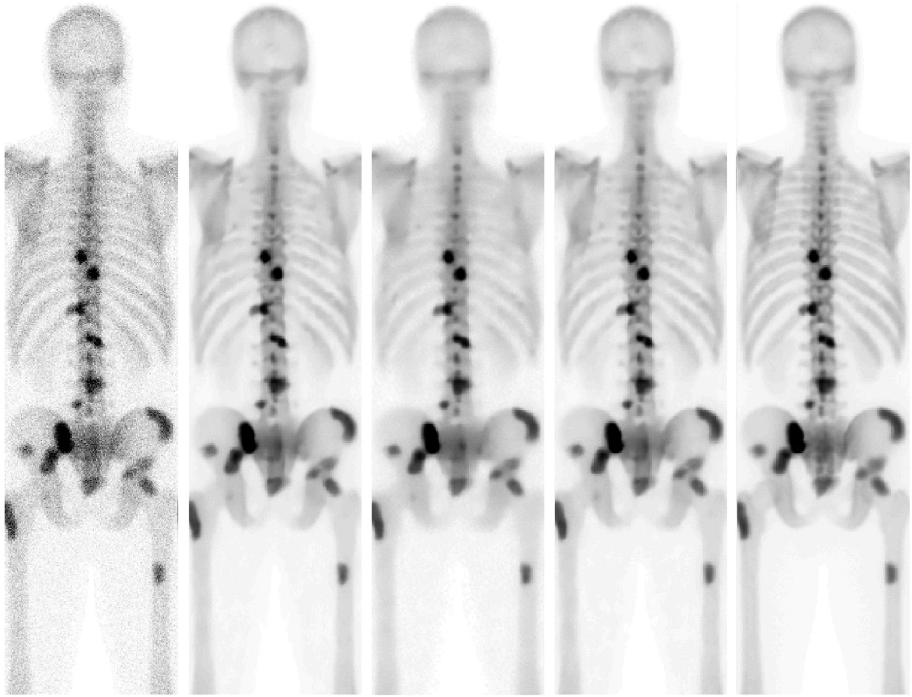
For each noisy and filtered image, the coefficient of variation was calculated for pixel values in a circular region of interest (109 pixels) placed in the homogeneous part of the middle of the phantom. The mean squared error (MSE) (Eq. 1) was calculated for each filtered and noisy image with the noiseless image as reference. Eq. 1where N and M are the matrix size in the x and y direction, n and m are the matrix indices of the image I. The CNNs were compared using 40 simulated bone scans that were not part of the training data. For each of the 40 bone scans, 10 images were created, which had different noise levels ranging from a total number of counts in the posterior view of 0.1 million to 1 million. All images were filtered with the CNNs, the gaussian, and median filters. The MSE was calculated for each filtered and noisy image, with the noiseless image as a reference. An example is shown in Figure 3.

Posterior view of simulation with 0.6 million counts. From left to right: noisy image; noisy image filtered with bone CNN, cylinder CNN, and mix CNN; and true image.
Clinical Evaluation
In a pilot clinical study, we compared mix CNN–filtered and gaussian-filtered (full width at half maximum, 7 mm) half-time imaging whole-body bone scans with standard scans. Images acquired with half the acquisition time were generated by binominal subsampling (21). Bone scans from 39 patients (3 women, 36 men) clinically referred to Skåne University Hospital, Malmö, Sweden, for assessment of bone metastases were evaluated. The median age was 76 y (range, 52–92 y). Patients were injected with 600 MBq of 99mTc-hydroxydiphosphonate. The accumulation time was 2–4 h. All patients were scanned on a Siemens Symbia γ-camera with a low-energy high-resolution collimator, a scan time of 15 cm/min, and a 256 × 1,024 matrix with a pixel size of 2.21 mm. One nuclear medicine physician (observer A) and 1 resident in nuclear medicine (observer B) interpreted the images in a random and masked fashion and assessed whether bone metastases were present. They were given only 1 set of images (anterior and posterior views) at a time and were not aware of their interpretation of the other image sets. After 2 mo, observer A reinterpreted the images. The presence of bone metastases was assessed separately for anterior and posterior views. The standard bone scans were considered the reference method. Sensitivity and specificity for detecting bone metastases for the CNN- and the gaussian-filtered images were calculated, as well as the area under the receiver-operating-characteristic curve. Differences between the standard and the CNN- and the gaussian-filtered images were assessed with the McNemar test using SPSS, version 25 (IBM).
Examples of bone scans and filtered equivalents are shown in Figure 4.
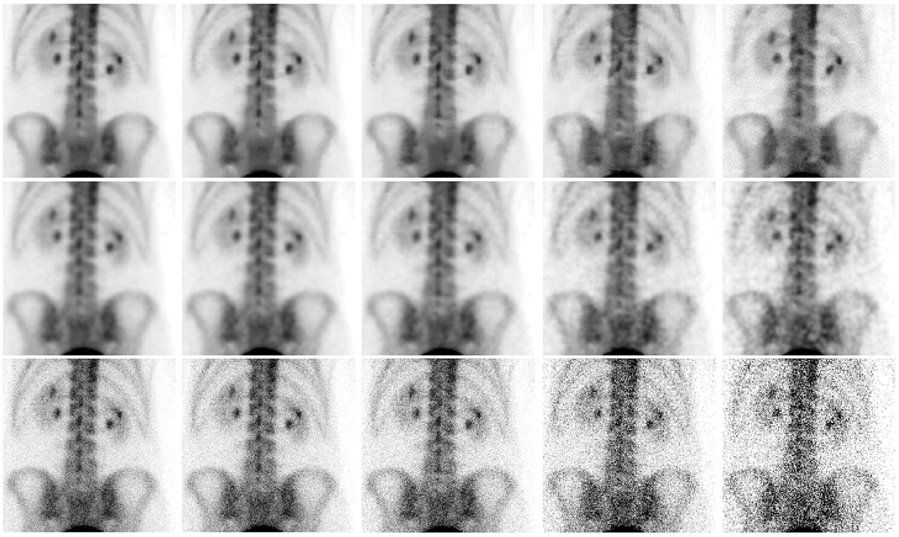
Posterior views of bone scan. From top to bottom: images filtered with mix CNN, images filtered with gaussian filter of 7 mm in full width at half maximum, and unfiltered images. From left to right: original images and images with 75%, 50%, 25%, and 10% of original counts.
The institutional review board at Lund University (2019-00644) approved this retrospective study, and the requirement to obtain informed consent was waived.
RESULTS
The calculation results of the coefficient of variation are displayed in Table 1, and the results of the MSE evaluation are presented in Tables 2 and 3. The best CNN reduced the coefficient of variation by, on average, 92%, whereas the best standard filter (mean filter with 81 pixels) reduced the coefficient of variation by 88%. The best CNN gave an MSE that was on average 68% and 20% better than the best standard filters (mean filter with 9 pixels and gaussian filter with a full width at half maximum of 7 mm), for the cylindric and bone scan images, respectively. The results showed that there was a small difference between images denoised with the different CNNs. The noise reduction in the specific case shown in Table 1 was more than 10-fold for the cylinder CNN and slightly less for the mix CNN. The cylinder CNN gave the lowest MSE in the evaluation with the cylindric phantom. For the bone scan evaluation, the best results were obtained for the bone CNN. The CNN created with a mix of images was similar to the best CNN for both cylindric phantom and bone scans. Among the conventional filters, a median filter with a 3 × 3 neighborhood and a gaussian filter with a full width at half maximum of 7 mm produced the best MSE results for the cylinder and bone scans, respectively.
Mean Coefficient of Variation in Percentage of 40 Noise Realizations
MSE Between Noisy and CNN-Filtered Cylindric Phantom Images with Noiseless Image as Reference
MSE Between Noisy and CNN-Filtered Simulated Bone Scan Images with Noiseless Image as Reference
The sensitivities, specificities, and areas under the receiver-operating-characteristic curve are found in Table 4. There were no significant differences between standard and CNN-filtered images (P = 0.99 and 1.0 for observer A and P = 0.25 for observer B) or between standard and gaussian-filtered images (P = 0.45 and P = 0.69 for observer A and P = 1.0 for observer B).
Performance of Filtered Images, Using Standard Bone Scans as Reference Method
DISCUSSION
We have trained and applied CNNs on simulated bone scans and images of cylindric phantoms. We have also used the CNNs to denoise real bone scans to verify the feasibility of using CNNs trained on Monte Carlo images to remove noise, and we performed a pilot clinical evaluation. We have shown that it is possible to achieve an almost total removal of noise with little or no resolution loss. The cylinder CNN even outperformed a median filter with a 9 × 9 neighborhood while still maintaining the resolution.
Other statistical filtering methods and other types of methods require some form of optimization of input parameters, which may not be valid for all intensity ranges encountered, such as those in bone scans. In contrast, a trained bone scan CNN can handle all types of scanning situations if the noise distribution in the training images follows that of real images and the range of intensities in the images reflects the whole spectra of observed intensities. This is demonstrated in Figure 4, which shows original bone scans, mathematically generated images representing the same image acquired with 75%, 50%, 25%, and 10% of the imaging time, and the corresponding CNN-filtered and gaussian-filtered images. There are some small structural differences between the CNN-filtered images, but the level of noise is almost the same, which is not case for the gaussian-filtered images. The 10% CNN-filtered image shows hot spots in the upper spine that are not seen in the images with higher count rates. Therefore, use of the CNN filter on images with only 10% of the counts might not be optimal, but this possibility needs to be established in future clinical studies.
It seems that the type of images used to train the CNN matters to some extent. The differences are most clearly seen in Figure 2, where the images filtered with the bone CNN are mottled. However, it seems that if a variety of images are used (e.g., a mix of different types of images), the result can be almost as good as if the CNN were trained using a specific set of images.
As with other filtering methods, it is necessary to establish whether the filtered images provide any benefits or improvements regarding the confidence about what the reading physicians see in the images. It is also necessary to establish that no false information is added to the images. In our pilot clinical evaluation, we showed that it is possible to reduce the scanning time by half and then apply the CNN filter and still obtain high accuracy for assessment of bone metastases. The observers were used to interpreting original bone-scan images, not CNN- or gaussian-filtered images. Since filtered images look different from original bone scans, the filtered images are not expected to increase reader confidence at this early stage. Whether CNN-filtered images can provide better accuracy in the detection of metastases than standard bone scans and whether the acquisition time can be further reduced need to be evaluated in larger clinical studies with a better ground truth than the standard bone scan.
It is crucial to have a good model for generating data used for training the CNN. Any error may lead to bias in the clinical images. Our study showed that it is possible to use Monte Carlo–simulated images for training the CNNs, if the training data are carefully generated. An alternative could be to use real bone scan images with high statistics as a substitute for noiseless images. However, to receive reasonably noiseless images, the imaging time needs to be long (more than 1 h) and few patients can lie completely still for such a long time. Therefore, we propose using Monte Carlo–simulated images instead.
CONCLUSION
Noise can be removed efficiently using a CNN trained with noisy and noiseless simulated images, regardless of the noise level and with little or no resolution loss. The CNN filter makes it possible to reduce the scanning time by half and still obtain good accuracy for detecting bone metastases, but confirmation in large clinical studies is needed.
DISCLOSURE
The work was made possible by research grants from the Knut and Alice Wallenberg Foundation, the Swedish Federal Government under the ALF agreement, Lund University, and Region Skåne. No other potential conflict of interest relevant to this article was reported.
KEY POINTS
QUESTION: Can a noise-reducing CNN be trained with Monte Carlo–simulated γ-camera images.
PERTINENT FINDINGS: The CNNs trained with Monte Carlo–simulated images were able to reduce noise by a factor of 10 while still maintaining the resolution.
IMPLICATIONS FOR PATIENT CARE: The results indicate that noise in planar nuclear medicine images can be removed efficiently with little or no resolution loss, thus enhancing the image quality and enabling shorter scanning times with preserved accuracy for detecting bone metastases.
Acknowledgments
We thank Anders Persson for interpretation of images.
Footnotes
Published online Jul. 19, 2019.
- © 2020 by the Society of Nuclear Medicine and Molecular Imaging.
REFERENCES
- Received for publication January 25, 2019.
- Accepted for publication July 8, 2019.


