


Abstract
Attenuation correction is important for PET reconstruction. In PET/MR, MR intensities are not directly related to attenuation coefficients that are needed in PET imaging. The attenuation coefficient map can be derived from CT images. Therefore, prediction of CT substitutes from MR images is desired for attenuation correction in PET/MR. Methods: This study presents a patch-based method for CT prediction from MR images, generating attenuation maps for PET reconstruction. Because no global relation exists between MR and CT intensities, we propose local diffeomorphic mapping (LDM) for CT prediction. In LDM, we assume that MR and CT patches are located on 2 nonlinear manifolds, and the mapping from the MR manifold to the CT manifold approximates a diffeomorphism under a local constraint. Locality is important in LDM and is constrained by the following techniques. The first is local dictionary construction, wherein, for each patch in the testing MR image, a local search window is used to extract patches from training MR/CT pairs to construct MR and CT dictionaries. The k-nearest neighbors and an outlier detection strategy are then used to constrain the locality in MR and CT dictionaries. Second is local linear representation, wherein, local anchor embedding is used to solve MR dictionary coefficients when representing the MR testing sample. Under these local constraints, dictionary coefficients are linearly transferred from the MR manifold to the CT manifold and used to combine CT training samples to generate CT predictions. Results: Our dataset contains 13 healthy subjects, each with T1- and T2-weighted MR and CT brain images. This method provides CT predictions with a mean absolute error of 110.1 Hounsfield units, Pearson linear correlation of 0.82, peak signal-to-noise ratio of 24.81 dB, and Dice in bone regions of 0.84 as compared with real CTs. CT substitute–based PET reconstruction has a regression slope of 1.0084 and R2 of 0.9903 compared with real CT-based PET. Conclusion: In this method, no image segmentation or accurate registration is required. Our method demonstrates superior performance in CT prediction and PET reconstruction compared with competing methods.
- CT prediction
- attenuation correction
- local diffeomorphic mapping
- outlier detection
- local anchor embedding
PET/MR systems have been used in a wide range of applications (1,2). MR intensities are not directly related to the attenuation coefficients that are needed for attenuation correction in PET imaging. Given that CT intensity is related to electron density, CT images are usually used in PET attenuation correction (3). Therefore, accurate prediction of CT images from MR images is highly desired for clinical applications.
Recently, various novel methods for predicting CT substitutes from MR data have been proposed. These methods are divided into 2 main categories: segmentation-based methods (4–7) and atlas-based methods (3,8–11). Segmentation-based methods usually classify voxels in MR images into different tissues and assign linear attenuation coefficients or CT values. Because standard MR images show low signals for bone structures, ultrashort echo time imaging, which enables imaging of bone structures with short T2 relaxation times (12), is highly preferred by many segmentation-based methods (4–6). However, segmentation of bone structures using ultrashort echo time images is still inaccurate in complicated regions such as the sinuses (3). Atlas-based methods usually perform deformable registration of training MR/CT pairs to the testing MR image, then use the deformed training CT images to help CT predictions (3,8,9). However, these methods usually involve the difficulty in precisely aligning each training MR/CT pair to the testing MR image. Of late, patch-based methods (12,13) have been proposed with promising results, in which similar patches between MR testing and training images are searched, and the corresponding CT training patches are combined to obtain CT predictions.
A patch-based method for predicting CT substitutes from given MR images is developed in this study. Considering that there is no global relation between MR and CT intensities, we assume MR and CT patches are located on 2 nonlinear manifolds and the mapping from the MR manifold to the CT manifold approximates a diffeomorphism under a local constraint. This study proposes local diffeomorphic mapping (LDM) to predict CT substitutes. A single intensity value cannot adequately represent the feature of 1 voxel in an MR image. An image patch contains more context information and has been proven effective in many studies (14,15). For a patch in the testing MR image, its similar patches in training MR images could be found in the nearby region. Therefore, we define a local search window in training MR/CT pairs to extract image patches to construct MR and CT dictionaries. In addition, k-nearest neighbors (kNN) (16) is used to strengthen the locality of the MR dictionary. To guarantee the locality in the CT dictionary, k-means clustering (17) and kNN are combined to detect outliers in the CT dictionary. Outlier corresponding samples in the MR dictionary are then deleted, generating a new MR dictionary to represent the testing MR patch. Local anchor embedding (LAE) (18) is performed to solve dictionary coefficients. Afterward, the dictionary coefficients are locally and linearly transferred from the MR manifold to the CT manifold and further used to combine samples in the CT dictionary to generate CT predictions. In the proposed LDM, image segmentation and accurate registration are not required. The proposed method is evaluated on brain data for 13 subjects in a leave-one-subject-out manner. Results show that the proposed method can obtain competitive CT predictions and PET reconstructions.
MATERIALS AND METHODS
Data Acquisition
Our dataset contains 13 healthy subjects, each with T1- and T2-weighted MR and CT brain images. T1-weighted MR images (echo time, 7.896 ms; repetition time, 2,884.7 ms; inversion time, 960 ms; flip angle, 90°; voxel size, 0.47 × 0.47 × 2.50 mm3) and T2-weighted MR images (echo time, 100.466 ms; repetition time, 5,000 ms; flip angle, 90°; voxel size, 0.47 × 0.47 × 2.50 mm3) were acquired on a Signa HDxt scanner (GE Healthcare). CT images (120 kVp; 240 mAs; voxel size, 0.47 × 0.47 × 2.52 mm3) were acquired on a LightSpeed Pro 16 scanner (GE Healthcare). This study was approved by the ethics committee, and a written informed consent form was obtained from each subject.
Data Processing
Necessary preprocessing was applied to all images. The N3 package was used to remove bias field artifacts from MR images. Intensities in each MR image were normalized to [0 100] based on a piecewise histogram-matching method (19). In each CT image, the head was separated from the bed using the thresholding technique as described in Burgos et al. (3). Afterward, all images were affinely registered to a common space in 2 steps. First, within each subject, we registered the subject’s T1 and T2 images to the CT image. Then, across individual subjects, we randomly selected a CT image of 1 subject as the common space to which all other subjects were further registered based on their CT images. Affine registration was performed by FMRIB’s linear image registration tool (FLIRT) (20) with mutual information as the similarity metric.
CT Prediction by LDM
Our goal can be described as follows: given a training dataset  containing N MR/CT patch pairs, how is the substitute CT patch
  of a testing MR patch
  calculated? LDM is based on 2 assumptions.
Assumption 1
Image patches from different modalities are located on different nonlinear manifolds, and a patch can be approximately represented as a linear combination of several nearest neighbors from its manifold.
In this paper, MR and CT manifolds are denoted as  and
and  , respectively. The column vector of patch
  (i.e.,
  ) can be linearly represented by its nearest neighbors on
  :
: Eq. 1
Eq. 1
 where
where  is a dictionary containing training MR patches.
  is the coefficient vector of
  .
.  is a set of K-nearest neighbors of
  in
in  .
.  denotes the reconstruction error. τ is a threshold that constrains
  under a small value.
Obviously, if the mapping f between  and
and  is explicitly known, the substitute CT patch
  of the testing MR patch
  can be calculated by
  . Given that obtaining an explicit formula of f is difficult, we suggest calculating
  in an implicit way. According to Equation 1, the column vector of patch
  (i.e.,
  ) can be written as:
 Eq. 2If f is linear, Equation 2 can be rewritten as:
 Eq. 3where
  contains vectorized training CT patches. Given that
  can be determined by Equation 1 and
  is given,
  can be calculated according to Equation 3.
The linearity of f is crucial in the derivation of Equation 3; thus, assumption 2 is introduced to support the above derivation.
Assumption 2
Under a local constraint, mapping from the MR manifold to the CT manifold f :  →
→ approximates a diffeomorphism.
The mapping f :  →
→ is called a diffeomorphism if it is differentiable and bijective, and its inverse
  :
:  →
→ is also differentiable. On the basis of assumption 2, a local region on
  can be linearly mapped onto a local region on
  by f. Therefore, Equation 3 can be derived. However, the mapping between MR and CT patches is not a diffeomorphism. For example, several materials have similar MR intensities but different CT values. Therefore, whether the structures in small MR and CT patches have a 1-to-1 correspondence remains uncertain. To solve this problem, several approaches are presented. The first approach is local MR and CT dictionary construction. For each testing MR patch, a local search window is used to preselect patches from training MR/CT pairs to construct MR and CT dictionaries. Furthermore, dictionary reselection and outlier detection are performed in MR and CT dictionaries, respectively, to further limit the dictionary elements in local regions. The second approach is local linear representation, wherein LAE is used to solve MR dictionary coefficients when representing the MR testing sample.
The proposed method contains 3 parts: local dictionary construction, local linear representation, and prediction. Detailed procedures are shown in Figure 1.

Detailed procedures of LDM.
Local Dictionary Construction
 is used to denote training images, where S and t are the number of training subjects and the image modality, respectively. For a testing subject Y, the T1 and T2 images are denoted as
  .
.
There are 3 steps in local dictionary construction. The first is dictionary preselection. Here,  is aligned to the space of I using FLIRT (20). Then, patches
  and
and  centered at point x in
  and
and  are extracted. We further vectorize
  and
and  to
to  and
and  , respectively, where m denotes the number of points in the image patch.
  and
and  are combined to denote the MR testing sample
  . For
. For  , a training dataset
  is collected. The center of each patch in T is constrained in a local search window centered at point x (red and green boxes in Fig. 1A). Each training patch pair {
 } is arranged to vectors {
 }, generating MR dictionary
  (red circles in Fig. 1B.1) and CT dictionary
  (green circles in Fig. 1B.1), where l denotes the number of points in the CT image patch. The second step is dictionary reselection. This step aims to constrain the MR dictionary in a local space, where kNN (16) is used to find k-nearest vectors of
  from
from  , thereby generating a new dictionary
  (red yellow circles Fig. 1B.2). On the basis of
  , k CT correspondences can be obtained in
  through pairs {
 }, generating
  . The third step is outlier detection. Outliers in CT dictionary are detected and deleted to constrain CT training samples in a local space. Various outlier detection methods are available, including density-based techniques (kNN) (16), local outlier factor (LOF) (21), one class support vector machines (OC-SVM) (22), and cluster-based methods (17). In our study, k-means clustering is combined with kNN to detect outliers in
  . The k-means is first used to obtain clustering centers in
  , and then kNN is used to find η-nearest samples of the clustering centers to generate
  (green yellow circles in Fig. 1B.3). Accordingly,
  is updated by deleting samples that correspond to the outliers in
  , generating
  (red yellow circles in Fig. 1B.3).
Local Linear Representation
This step aims to seek  when representing testing sample
  based on
  , that is,
  . Various techniques for solving the dictionary coefficients are available. Sparse coding with least absolute shrinkage and selection operator (LASSO) (23) uses several training samples with nonzero coefficients to linearly represent the testing sample. Locality-constrained linear coding (LLC) (24) focuses on locality by limiting linear coding within a local space. In LAE (18), the reconstructed sample is located in a convex region on a hyperplane spanned by its closest neighbors:
 Eq. 4
Eq. 4

 where
where  is a set of K-nearest neighbors of
  in
in  . Given that locality is important in this study, LAE is used to solve the dictionary coefficients.
Prediction
The CT correspondence of  (i.e.,
  ) can be generated on the basis of Equations 2–4:
 Eq. 5Vector
  can be reshaped into a CT patch
  (green grid in Fig. 1D) centered at point x. After predicting a CT patch for each point, the weighted average of overlapped patches is obtained to achieve the CT value at each point. The weight of point u in patch
  is defined according to the distance from u to x:
 Eq. 6where
  is the Euclidean distance between u and x. As u gets away from x, the weight at u decreases, indicating that the patch contributes more in predicting central points than peripheral points.
Finally, the predicted CT value of point x is calculated via: Eq. 7where u is a point in patch
  ,
,  is the weight of x in patch
  , and
, and  is the intensity value of x in patch
  . Given that the image patch centered at u (i.e.,
 ) covers point x, we weight-averaged all overlapped CT patches at x (i.e.,
  ) to obtain
  (green solid circle in Fig. 1D).
PET Reconstruction
After CT prediction, the predicted CT images are transformed to attenuation coefficient maps (μ-map) based on the following criteria (12): Eq. 8where h denotes the CT value in Hounsfield units (HUs).
Our dataset does not contain PET scans. To apply the proposed method in PET attenuation correction, we followed Hofmann et al. (11) to simulate a PET image for each subject. The template brain MR and 18F-FDG PET images in statistical parametric mapping toolbox (25) were used, and the MR template in the toolbox was registered to each subject in our dataset using Advanced Normalization Tools (26). The obtained deformations were further applied to the PET template, generating a PET image for each subject. The attenuation correction was performed the same way as in Hofmann et al. (11).
Evaluation
Validation Scheme
This method was evaluated in a leave-one-subject-out manner, in which 12 subjects were used as the training data and the remaining subject was regarded as the testing data. A set of experiments was performed: accuracy of predicted CTs compared with real CTs, effectiveness of considering locality, performance of using multimodality MR images, comparison of relevant methods in CT prediction and PET reconstruction. The Wilcoxon signed-rank test was used to show the statistical result between each compared method and the proposed method.
The predicted CT was compared with the real CT by 4 measures: the mean absolute error (MAE) for voxels in the brain volume, Pearson linear correlation coefficient, peak signal-to-noise ratio (PSNR), and Dice similarity coefficient (DSC) of bone volume. The bone region was obtained by setting a threshold at 100 HUs as in Burgos et al. (3).
Accuracy of PET reconstruction was measured by the coefficient of determination R2 and the linear regression slope from scatterplots.
Parameter Selection
A 2-fold cross-validation strategy was used to choose parameters. Specifically, the dataset was randomly divided into 2 groups consisting of 6 and 7 subjects, respectively. To determine the parameters in 1 group, we performed leave-one-out cross-validation on the other group. The parameter combination that resulted in the lowest average MAE was chosen. Finally, we set the MR patch size to 15 × 15 × 3 (first group) and 13 × 13 × 3 (second group), local search window to 17 × 17 × 5 (both groups), number of nearest neighbors in LAE (i.e., K in Eq. 4) to 30 (first group) and 40 (second group), and parameter a in Equation 6 to 0.9. In outlier detection, 1 clustering center in k-means was chosen, and 70% of samples in the CT dictionary were retained via kNN. Note that 3 parameters were set empirically and were not included in the cross-validation: 1.0 and 1.2 for the weights of T1 and T2, respectively (i.e.,  ); 100 for the number of nearest neighbors in kNN in dictionary reselection; and 3 × 3 × 1 for the size of the predicted CT patch (i.e.,
  ).
).
RESULTS
Accuracy of CT Prediction
The mean ± SD of MAE, correlation, PSNR, and bone DSC for all subjects comparing CT substitutes with real CTs were 110.1 ± 15.3 HUs, 0.82 ± 0.11, 24.81 ± 2.18 dB, and 0.84 ± 0.03, respectively. Figure 2 shows CT prediction results of 3 slices from different subjects. Columns 1–5 correspond to T1, T2, real CT, predicted CT, and difference images between real and predicted CTs, respectively. The upper scale bar shows the intensity distribution of real and substitute CTs, whereas the lower scale bar shows the values in difference images. In difference images, red indicates a higher intensity in the real CT and blue indicates a higher intensity in the CT substitute. Large differences between real and substitute CTs are present at tissue interfaces and in bone regions.
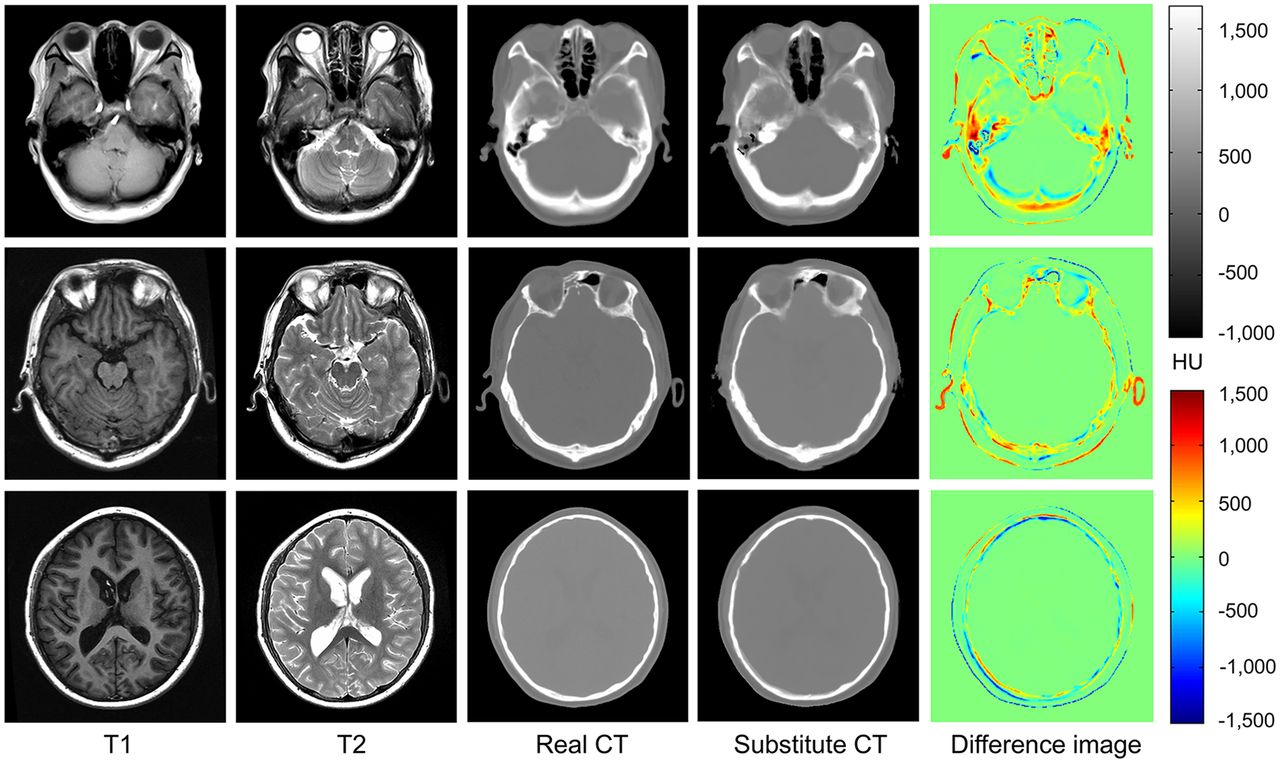
CT prediction results by the proposed method. MAEs of 3 slices are 140, 85, and 53 HUs; PSNRs are 21.6, 22.5, and 24.7 dB; correlations are 0.83, 0.84, and 0.83; and bone DSCs are 0.88, 0.86, and 0.88 from row 1 to 3.
Effectiveness of Considering Locality
k-means + kNN in Outlier Detection
In this section, OC-SVM (22), LOF (21), and k-means combined with kNN (i.e., k-means + kNN) are compared. Figure 3A shows the mean ± SEM of MAEs for 13 subjects obtained by OC-SVM, LOF, and k-means + kNN in outlier detection. Compared with OC-SVM and LOF, k-means + kNN obtains 3.5 and 2.4 HU lower mean MAEs than OC-SVM (P = 0.0061) and LOF (P = 0.0415). To evaluate the effectiveness of the outlier detection step, results of the method without outlier detection are also shown in Figure 3A. Compared with the method without outlier detection, the mean MAE of 13 subjects obtained by k-means + kNN was reduced from 117.9 to 110.1 HUs (P = 0.0002).
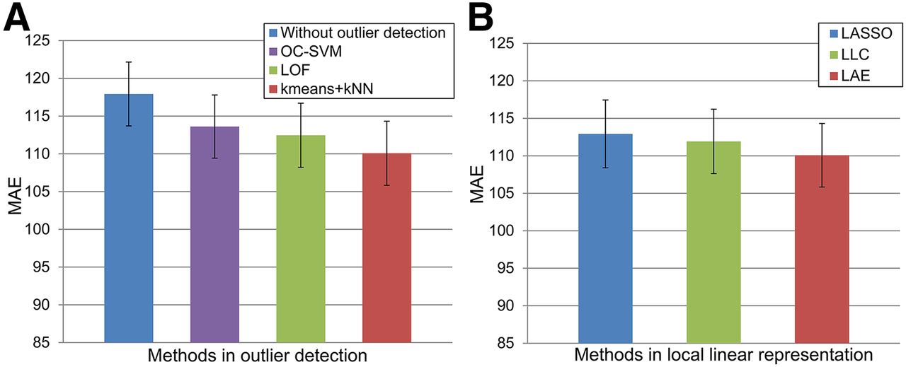
Effectiveness of considering locality: mean ± SEM of MAE for 13 subjects obtained using OC-SVM, LOF, and k-means + kNN in outlier detection, as well as method without outlier detection (A) and mean ± SEM of MAE obtained using LASSO, LLC, and LAE to solve dictionary coefficients (B).
LAE in Local Linear Representation
Three coding methods (i.e., LASSO, LLC, and LAE) were compared for selection to solve dictionary coefficients. Figure 3B shows mean ± SEM of MAEs for 13 subjects obtained by different coding techniques. Compared with LASSO, the mean MAE across all subjects using LAE was reduced from 112.9 to 110.1 HUs (P = 0.0256). Compared with LLC, LAE obtained a 1.8 HU lower mean MAE (P = 0.0112).
Performance of Using Multimodality MR Images
To show the impact of using different modalities, performance was evaluated using only T1 or T2 or combined T1 and T2. Figure 4 shows the results of 2 slices obtained using T1, T2, and T1 + T2. The mean ± SD MAEs obtained using T1, T2, and T1 + T2 were 119.8 ± 15.9, 118.9 ± 16.7, and 110.1 ± 15.3 HUs, respectively. Using both T1 and T2 produces better results than a single T1 (P = 0.0002) or T2 (P = 0.0034). When a single-modality MR image (T1 or T2) was used, there was no statistically significant difference between the results (P = 0.6956).

Results of 2 slices (A and B) generated using T1, T2, and T1 + T2 images. MAEs for the 2 slices obtained using T1/T2/T1 + T2 are 131/132/124 HUs (A) and 89/81/77 HUs (B), PSNRs are 21.1/21.0/21.7 dB (A) and 21.8/22.2/22.8 dB (B), correlations are 0.82/0.81/0.84 (A) and 0.74/0.68/0.75 (B), and bone DSCs are 0.80/0.81/0.82 (A) and 0.76/0.74/0.82 (B).
Comparison of CT Prediction
LDM is compared with 3 relevant methods (i.e., Burgos et al. (3), Ta et al. (27), and Andreasen et al. (13)). Burgos et al. (3) considered local information and used the local image similarity measure to match each MR/CT pair to a given MR image to predict CT substitutes. Ta et al. (27) combined patch-matching (28) with label fusion (14) in the segmentation task. This method (27) found k similar patches of the testing patch from the training dataset and weight combined the training labels by calculating the sum of the squared difference between testing and training patches. Ta et al.’s method can be applied in CT prediction by replacing label fusion with CT intensity fusion. Andreasen et al. (13) proposed a patch-based method, where k-nearest patches between MR testing and training images were searched and the corresponding CT training patches were combined to obtain the CT prediction. Because the input testing MR image is a single image in Burgos et al. (3), these methods are compared using T1 or T2 as the testing MR image. Results measured in MAE, correlation, PSNR, and bone DSC by 4 methods are shown in Table 1. Our method achieves better results than each of the compared methods. The P values of the Wilcoxon signed-rank test are also shown in Table 1.
In our study, a server with 32 cores at 2.13 GHz and 128-G memory was used. Because each patch can be processed independently, we used parallel processing to speed up our algorithm. For CT prediction of 1 subject, our algorithm took 2.8 h on average. Burgos et al. (3), Andreasen et al. (13), and Ta et al. (27) took approximately 2.5 h, 2.3 h, and 45.1 min, respectively.
Comparison of PET Reconstruction
Figure 5 shows the results of 1 slice obtained by 4 methods using T1 (rows 1–3) and T2 (rows 4–6). Visually, LDM produces the closest μ-maps to the real CT μ-map; however, PET reconstructions from all methods look similar. Scatterplots are used for this slice to compare intensities of PET images reconstructed from predicted and real CTs (Supplemental Fig. 1; supplemental materials are available at http://jnm.snmjournals.org). The dashed red lines indicate a linear fit for all points. The slope of dashed lines should ideally be 1. As can be seen from Supplemental Figure 1, all 4 methods produce satisfactory results, and the slope of LDM is closest to 1 when using T1 or T2.
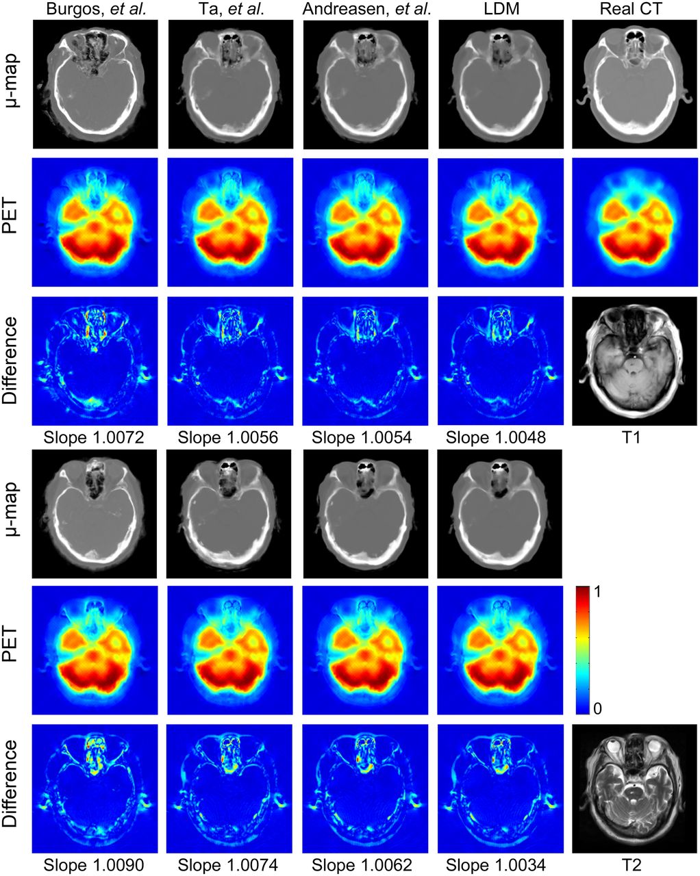
Results generated by Burgos et al. (3), Ta et al. (27), and Andreasen et al. (13), and LDM based on T1 (1–3 rows) or T2 (4–6 rows) image. First and fourth rows show μ-maps. Second and fifth rows show reconstructed PET images from different μ-maps. Third and sixth rows show absolute difference images between PET images reconstructed by predicted CTs and real CTs. Values in difference images are 5 times as original differences.
The accuracy for PET reconstruction from different μ-maps measured in regression slope and R2 from scatterplots for all subjects are shown in Table 2. LDM generates the best results for slopes and R2 on T1 or T2 images. When using both T1 and T2, LDM obtained a mean ± SD slope of 1.0084 ± 0.0182 and R2 of 0.9903 ± 0.0051 from scatterplots.
Mean ± SD of Regression Slope and R2 from Scatterplots for 13 Patients Obtained by Comparing Intensities of PET Images Reconstructed from Predicted and Real CTs
DISCUSSION
There are 2 assumptions in the current study. Assumption 1 has been successfully applied in classification studies (15,29,30), in which the samples from different classes are located on different nonlinear submanifolds and a sample can be approximately represented as a linear combination of several nearest neighbors from its corresponding submanifold. Considering that samples from MR and CT belong to different classes and should be located on different nonlinear manifolds, we applied this assumption to the current study. Assumption 2 is crucial and is used to derive Equation 3. However, the mapping between MR and CT samples is not a diffeomorphism without any constraint. To solve this problem, we emphasized the locality using local dictionary construction and local linear representation. Under these local constraints, the selected MR and CT training samples are expected to have a 1-to-1 correspondence, which supports assumption 2.
In our experiments, we showed the results using different outlier detection techniques (i.e., OC-SVM, LOF, and k-means + kNN). Both kNN and LOF belong to density-based techniques and produced lower prediction errors than OC-SVM, indicating that density-based techniques are more suitable for our dataset. In LOF, because no definite rule exists to determine whether a sample is an outlier, this may lead to incorrect detections in our dataset. k-means + kNN produced the best results and was chosen in the current study. In addition, we showed the performance of different coding techniques. LAE and LLC emphasize the locality of the representation and generate lower prediction errors than LASSO, reaffirming the importance of considering locality in this study. Compared with LLC, LAE ensures the reconstructed sample is a convex combination of its K-nearest neighbors and is more suitable in this study.
In our experiments, we compared techniques with Burgos et al. (3), Ta et al. (27), and Andreasen et al. (13). For Burgos et al. (3), we used their online implementation on the Translational Imaging Group website. The results of Burgos et al. (3) in our experiments are worse than what they reported, possibly the result of the difference in data used in our respective studies. Parameters in Ta et al. (27) and Andreasen et al. (13) were optimized in the same way as the proposed method. Compared with our previous study (31), in this paper, parameters were further optimized, the accuracy of CT prediction was further validated, and the application in PET attenuation correction was added.
In our method, we did not apply deformable registration but used only affine registration (i.e., FLIRT) to align images. Because our dataset contains only brain images, we assumed that there are only small deformations between T1, T2, and CT images for the same patient. For deformations between different subjects, we used a large search window to select training samples, and only similar samples were retained after dictionary reselection and outlier detection. This process is supposed to solve the problem caused by inaccurate alignment between different subjects. However, when studying body images, we need to replace FLIRT by deformable registration methods, because large deformations may exist between T1, T2, and CT images of the same patient due to respiration.
Errors at tissue interfaces are possibly caused by the low intensities in conventional MRI sequences (i.e., T1 and T2 images) in both bones and air. In bone regions, 2 MR patches with similar low intensities may correspond to 2 CT patches with vastly different CT values and this may be one of the causes for high prediction errors in bone regions. More image information in bone structures may improve the prediction accuracy at tissue interfaces and in bone regions.
The proposed method does not require image segmentation or accurate registration. Compared with existing patch-based methods, we proposed to emphasize the locality in both MR and CT dictionaries. Outliers were detected in the CT dictionary, and LAE was used to solve dictionary coefficients. Results indicate that emphasis on locality can significantly improve the accuracy of CT predictions.
Although the proposed method has several advantages, it still has a few limitations: because of the limited information provided by conventional MR images, errors at tissue interfaces and in bone regions still exist; as with all atlas-based methods, the proposed method requires a dataset containing MR/CT pairs; and computation time needs to be improved.
Future work includes adding other MRI sequences, which may provide a better estimate on bone density. Because all subjects are healthy volunteers, we can also add subjects with abnormal anatomies to further evaluate this method in pathologic states. Finally, speeding up the proposed algorithm is a part of our future work.
CONCLUSION
This paper presents a patch-based method for CT prediction from MR images, which can be applied to brain PET attenuation correction. In LDM, we assume MR patches and CT patches are located on different nonlinear manifolds, and the mapping from MR to CT manifold approximates a diffeomorphism under a local constraint. Several techniques are performed to construct local dictionaries (i.e., local search window, kNN in MR dictionary, and outlier detection in CT dictionary) whereas LAE is used in local linear representation. Under these local constraints, the MR dictionary coefficients are linearly transferred to the CT manifold to generate CT predictions. No image segmentation or accurate registration is required. The proposed method is evaluated for brain images on a dataset of 13 MR/CT pairs and demonstrates superior performance compared with competing methods.
DISCLOSURE
The costs of publication of this article were defrayed in part by the payment of page charges. Therefore, and solely to indicate this fact, this article is hereby marked “advertisement” in accordance with 18 USC section 1734. Financial support for this work was provided by the National Natural Science Funds of China (61471187, U1501256), Guangdong Provincial Key Laboratory of Medical Image Processing (2014B030301042), Pearl River Young Talents of Science and Technology in Guangzhou (2013J2200065), and Excellent Young Teachers Program of Guangdong Colleges. No other potential conflict of interest relevant to this article was reported.
Footnotes
Published online May 26, 2016.
- © 2016 by the Society of Nuclear Medicine and Molecular Imaging, Inc.
REFERENCES
- Received for publication July 22, 2015.
- Accepted for publication April 16, 2016.


Jump to section
Related Articles
Cited By...
- No citing articles found.