


Abstract
Tumor standardized uptake values (SUVs) vary with the interval between 18F-FDG injection and image acquisition. This paper presents a simple method using a single reference point to make appropriate time corrections for tumor SUVs. Methods: The reference point method was algebraically deduced from observations made by Beaulieu et al., who found that tumor SUVs behaved linearly over time (∼30 to 75 min after 18F-FDG injection). Eighteen patients with breast cancer were dynamically examined with PET/CT (∼60 and 80 min after 18F-FDG injection). Maximum SUV was calculated by applying 2 different iterative reconstruction methods (high-definition reconstruction and attenuation-weighted ordered-subsets expectation maximization). Reference points for time corrections were given, and errors for corrections obtained with the reference point method were calculated. Results: Variations in the reconstruction algorithm strongly influenced the coordinates of the reference point. Time corrections using the reference point method were more accurate at higher tumor SUVs (>8 at high-definition reconstruction and >6 at attenuation-weighted ordered-subsets expectation maximization) than at lower ones. Conclusion: A common origin of tumor SUVs over time exists in breast cancer. In combination with the linear behavior of tumor SUVs between approximately 30 and 80 min, such a reference point allows for straightforward time corrections of tumor SUVs. Parameters for image reconstruction must be considered because they influence the coordinates of the reference point.
- fluorodeoxyglucose (FDG)
- positron emission tomography (PET)
- standardized uptake value (SUV)
- exposure time
- breast cancer
Uptake of 18F-FDG in malignant tumors is subject to many influencing factors. Actual uptake is determined not only by the avidity of the tumor for 18F-FDG and its ability to store 18F-FDG but also by a variety of factors not directly relating to the tumor. Thie (1) mentioned 8 categories of confounding factors—that is, non–tumor-related factors—that influence 18F-FDG uptake. The interval between 18F-FDG injection and image acquisition (exposure time) is among the most important. The dependence of tumor standardized uptake values (SUVs) on exposure time relates to the ability of most tumors to accumulate 18F-FDG.
In clinical practice, uptake of 18F-FDG by tumors is reflected by the SUV obtained from 18F-FDG PET or PET/CT images. Surprisingly, there are only few references about how to correct the SUV for different exposure times to 18F-FDG whereas there are numerous suggestions about how to correct for other factors such as interindividual body tissue composition or different levels of blood glucose (2,3). Hamberg et al. (4) were among the first to report that 18F-FDG uptake in malignant tumors does not level off until several hours after injection—a feature that has since been confirmed for a variety of tumor entities (5). Wong et al. (6) proposed a power function to approximate 18F-FDG uptake over a limited time range. Complex methods of correcting 18F-FDG uptake for different exposure times have been suggested (1,6,7).
Beaulieu et al. (8) reported that SUVs in breast cancer are linear between approximately 30 and 75 min after injection. In addition, those authors gave a method by which users could correct SUVs for different exposure times to 18F-FDG. That method relies on data triplets that relate tumor SUVs at fixed time points after 18F-FDG injection to a certain slope and intercept of SUV changes over time—allowing estimation of SUVs at different time points (8). The need to correct tumor SUVs for time is of particular importance when tumor SUVs are being compared between different institutions or between baseline and follow-up (e.g., therapy monitoring).
This study is based on the findings of Beaulieu et al. (8) and their suggested correction method of tumor SUVs for different exposure times. In particular, their observation of a double linear relationship for tumor SUVs was fully adopted for this study. The aims of this study were to simplify Beaulieu's method using a single reference point—referred to as the reference point method—and to implement this simplified method in a patient cohort with breast cancer.
MATERIALS AND METHODS
Time Correction According to Beaulieu
As found by Beaulieu et al. (8), there is a double (primary and secondary) linear relationship between SUVs in breast cancer and time after 18F-FDG injection. The primary linear relationship regards the time course of individual tumor SUVs between approximately 27 and 75 min after injection, according to:
The method of Beaulieu et al. (8) to correct for different exposure times is based on 4 exemplary secondary linear relationships (intercepts a′ and slopes b′) belonging to 4 exemplary fixed time points for SUV measurements (t0 = 27, 42, 57, and 71–75 min) resulting in 4 data triplets (t0, a′, b′). Based on any tumor SUV measured—for example, after 60 min—the user could compare the measured time point with the fixed time points t0 given by Beaulieu et al.; choose, interpolate, or extrapolate the most appropriate data triplet (i.e., the corresponding intercept a′ and slope b′); and calculate the individual slope bi of the time course belonging to the measured SUV according to Equation 2. With this individual slope at hand, the user could calculate any tumor SUV over time based on the measured tumor SUV. The reference point method is based on the method of Beaulieu et al. to correct for time effects on tumor SUVs.
Patients
Eighteen consecutive women with histopathologically confirmed breast cancer were examined with PET/CT. Only patients with a primary diagnosis of breast cancer before any kind of therapy were included. All patients signed an informed consent form before the injection of 18F-FDG. This was a retrospective study performed in accordance with the regulations of the local ethics committee and federal laws.
Dynamic 18F-FDG PET/CT Scans
Dynamic 18F-FDG PET/CT scans were obtained on a Biograph mCT (Siemens Molecular Imaging). The system consisted of a full-ring dedicated PET scanner equipped with lutetium oxyorthosilicate crystals and a 2 × 64-slice spiral CT scanner. The axial field of view of the PET detector was 21.8 cm (9).
All patients were instructed to fast 6 h before receiving an intravenous bolus injection of 18F-FDG (mean ± SD, 270 ± 35 MBq; range, 220–350 MBq). Patients with a blood glucose level exceeding 150 mg/dL were not included in the study. Dynamic PET imaging over 20 min was started about 60 min after 18F-FDG injection. A single bed position was obtained in 3-dimensional list mode covering an area from the upper thorax to the upper abdomen, with the breast tumor being in a central position. CT was acquired using low-dose technique for attenuation correction.
Dynamic, attenuation-corrected PET images were rebinned into five 4-min intervals applying a 128 × 128 matrix (pixel length, 4.1 mm) and a slice thickness of 5 mm. Two different image reconstruction algorithms were applied. The first, high-definition, was based on attenuation-weighted ordered-subsets expectation maximization (OSEM) using 3 subsets and 24 iterations and additionally used a modulation of the point spread function in order to increase reconstructed spatial resolution (10). A 3-dimensional gaussian filter of 2.0 mm in full width at half maximum was applied (10). The second reconstruction algorithm was attenuation-weighted OSEM using 4 subsets with 18 iterations and a gaussian filter of 4 mm in full width at half maximum.
Image and Data Analysis
Scans were displayed in 3 orthogonal planes (axial, coronal, and sagittal), and tumor volumes of interest were manually confined to the tumors using the view tool of the PMOD 3.0 software package (PMOD Technologies Ltd.). Maximum SUVs were calculated according to the standard formula using body weight as a surrogate for the distribution volume of 18F-FDG. Data were further analyzed and graphs generated with SigmaPlot 11.0 (Systat Software GmbH). In lesions smaller than 3 times the overall spatial resolution (4 mm for high-definition reconstruction, 5 mm for attenuation-weighted OSEM) within the reconstructed images, partial-volume correction was applied according to Jentzen (11) using the maximum-based recovery correction approach. For statistic comparisons, a Wilcoxon signed rank test was applied at a significance level of P = 0.05.
RESULTS
It can algebraically be shown—as the nucleus of this work—that all individual SUV courses over time that obey the double linear relationship found by Beaulieu et al. (8) intersect at a single point when extrapolated toward smaller time points. This point of intersection, or reference point, allows for straightforward time correction of measured SUVs by the drawing of a line between the reference point and the measured SUV (Fig. 1). Only this single reference point with a time and an SUV coordinate (tref and SUVref, respectively) is necessary to make the desired time corrections. No interpolation or extrapolation is needed for the reference point method. Algebraically, any desired SUV can be calculated along the reference point method according to:
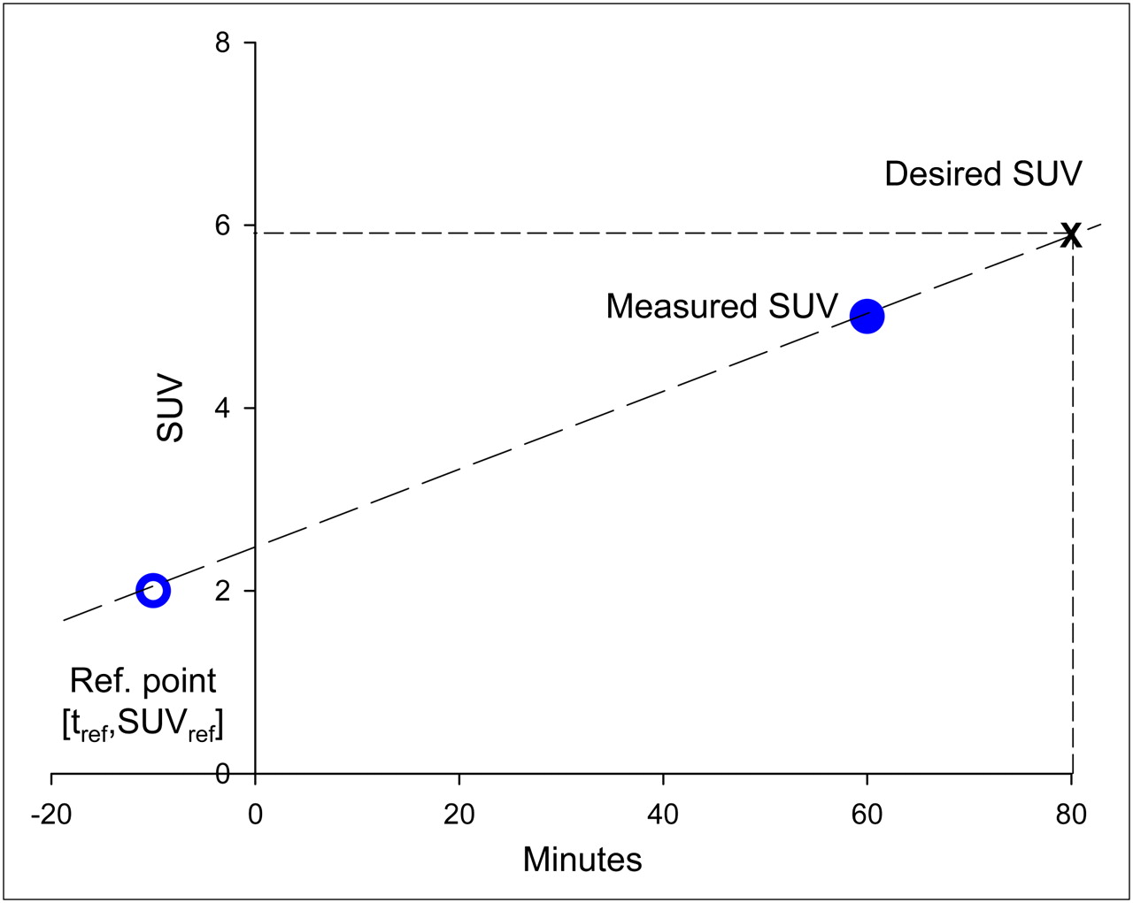
Illustration of reference point method for time corrections of tumor SUVs. Connect reference point (open circle with coordinates tref and SUVref) and measured SUV (filled circle) with a line. The line represents any desired SUV at a certain time point (e.g., at the cross hair).
The algebraic deduction of the reference point method is given in detail in the supplemental data (supplemental materials are available online only at http://jnm.snmjournals.org). The final formulas from this algebraic deduction are for tref and SUVref:
The reference point for the application of this method can be calculated from any given dataset of SUVs that corresponds to the double linear relationship according to Beaulieu et al. (8). Table 1 contains the reference points found in this study and those calculated from Beaulieu et al. (8).
Reference Points for Different Reconstruction and Analysis Approaches
Evaluation of Reference Point Method for Tumor SUVs in Breast Cancer
In 18 patients (mean age ± SD, 55 ± 12 y) the mean size of primary breast carcinomas was 21 ± 6 mm (range, 12–36 mm). The maximum recovery coefficients applied for partial-volume correction ranged from 0.46 to 1.00. Patients were imaged from 63 ± 10 to 83 ± 10 min after injection. SUVs over time for individual patients and reconstruction algorithms are given in Figure 2. As already shown for time points between about 27 and 75 min by Beaulieu et al. (8), most tumors showed an approximately linear increase in SUV; some tumors with rather low SUVs showed no increase or even a slight decrease in SUV over time.
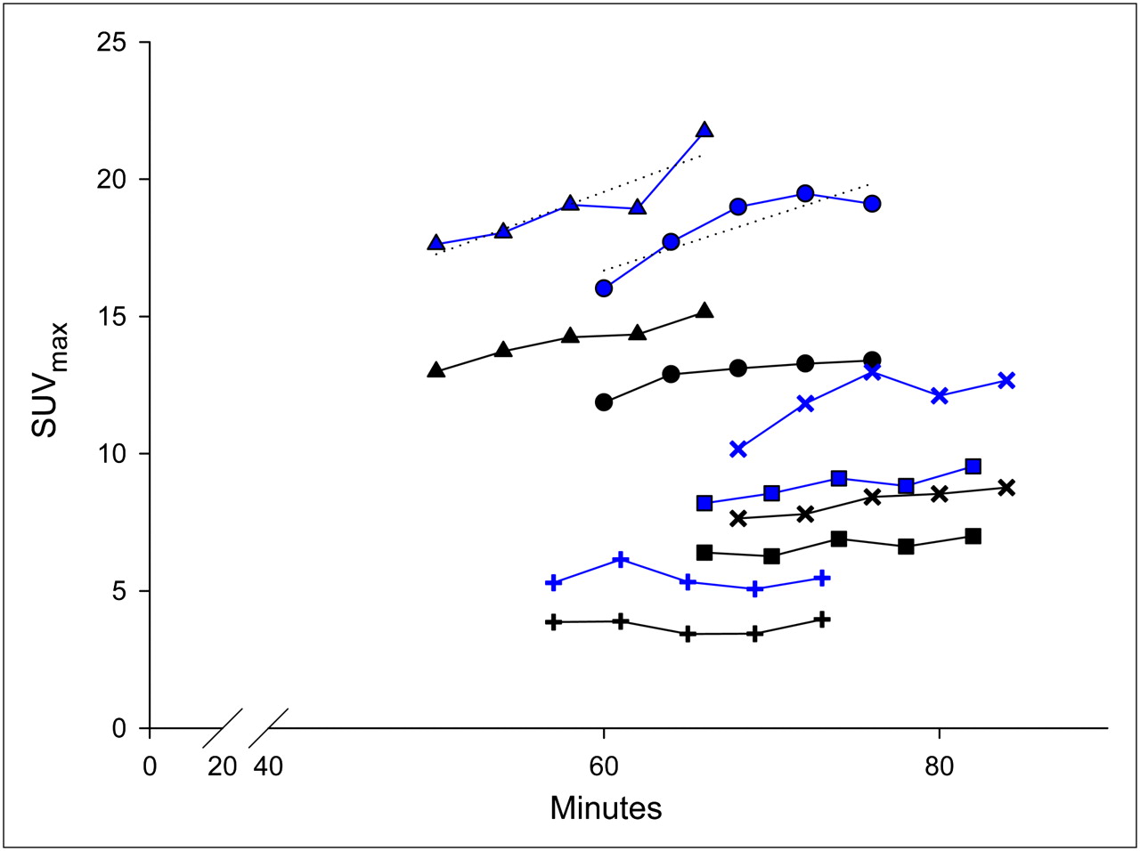
Maximum SUVs obtained from individual breast carcinomas over time. Two curves (same symbols) are denoted for each carcinoma, with upper curve representing high-definition reconstruction and lower curve representing attenuation-weighted OSEM. To allow for further calculation, regression lines were determined for each curve; examples are shown for the top 2 curves in the figure.
A regression analysis of the respective individual SUV course was performed to obtain the individual intercept ai and slope bi (examples are shown in Fig. 2) of the primary linear relationship of tumor SUVs over time. With these data, for each patient a representative SUV at a fixed time point t0 = 60 min after injection was calculated according to Equation 1. Figure 3 plots the representative SUVs at 60 min against the rate of SUV changes (bi) for each patient, for the 2 different reconstruction algorithms. An underlying secondary linear relationship between SUVs at 60 min and bi is evident (R2 = 0.82 and R2 = 0.73 for high-definition reconstruction and attenuation-weighted OSEM, respectively), as already shown by Beaulieu et al. (8). With the intercept a′ and slope b′ of this secondary linear relationship as well as t0 = 60 min, the reference points for both reconstruction algorithms—high-definition and attenuation-weighted OSEM—were calculated using Equations 4 and 5 (Table 1).
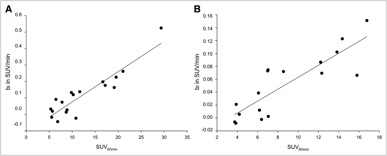
High-definition reconstruction (A) and attenuation-weighted OSEM (B). Shown are secondary linear relationship between SUVs at fixed time points (SUV at 60 min) and corresponding rates of change in SUV (slope bi). Resulting correlation had regression coefficients of R2 = 0.83 and R2 = 0.72, respectively.
As a next step, we calculated the errors that occurred with the reference point method versus no correction. For this purpose, the SUVs measured at the last time point of the dynamic series were compared with SUVs measured at the first time point, that is, approximately 60 min versus 80 min and vice versa (Table 2). Figure 4 plots the absolute percentage errors for both approaches (reference point method vs. no correction) and both reconstruction algorithms. A clear advantage for reference point method correction versus no correction was seen at high SUVs (i.e., >8 for high-definition reconstruction and >6 for attenuation-weighted OSEM)—that is, on average 5.8% versus 14.0% absolute error for high-definition and 4.8% versus 9.5% for attenuation-weighted OSEM (P < 0.01), whereas at low SUVs no such advantage was seen (Fig. 4).
Errors Associated with Time Corrections

High-definition reconstruction (A) and attenuation-weighted OSEM (B). Percentage error (absolute values) is plotted against maximum SUV when no correction for time differences in maximum SUV was applied (•; latest vs. earliest time point and vice versa) and when time corrections according to reference point method were applied (○). Percentage errors for both methods were fitted with linear function and peak function type Weibull, respectively. Above maximum SUV of approximately 8 and 6 for high-definition reconstruction and attenuation-weighted OSEM, respectively, reference point method had clear advantage over no correction.
Finally, we examined the influence of background activity on the secondary linear relationship by subtracting mediastinal activity (maximum SUV) from tumor SUVs. With this adjustment, the secondary relationship was preserved but the grade of correlation between background-corrected SUV at 60 min and the individual slopes of the SUV time courses was not improved (R2 = 0.85 and R2 = 0.67 for high-definition reconstruction and attenuation-weighted OSEM, respectively). However, the SUV coordinates of the reference points were smaller when background correction was used (Table 1).
DISCUSSION
The nucleus of this study was the recognition of a characteristic property of tumor SUVs in breast cancer—a property in addition to the primary linear course of tumor SUVs over time (within clinically common imaging time points) and the secondary linear relationship between individual SUV slopes and measured tumor SUVs at fixed time points as shown by Beaulieu et al. (8). This newly found property was the existence of a common point of intersection for all primary linear SUV courses over time when they are extrapolated toward smaller time points. The existence of this common point, or reference point, was algebraically deduced from the results of Beaulieu et al. without any additional experiments. Furthermore, no information from Beaulieu et al. (8) was lost, nor was any information added.
The existence of a reference point for all individual SUV courses strongly simplifies time corrections of SUVs. Any virtual tumor SUV between about 30 and 80 min after 18F-FDG injection can now be calculated by the simple drawing of a line between the reference point and the measured tumor SUV (Fig. 1). Results using the reference point method for time corrections are not different from results using Beaulieu's method because both methods are algebraically equivalent. However, the reference point method avoids extrapolation or interpolation and is straightforward. Interestingly, Beaulieu has also given a single-equation method for time correction (actually it is a 2-step procedure) but without taking advantage of the simple 1-point reference lying behind his findings.
The breast cancer patient cohort investigated here served as an example for testing the reference point method. For this purpose, common PET reconstruction and SUV calculation were applied—that is, iterative reconstruction (high-definition and attenuation-weighted OSEM) and calculation of maximum SUV—and corresponding reference points according to the reference point method were calculated. Our study was not intended to confirm or refute the double linear relationship of tumor SUVs in breast cancer as found by Beaulieu et al. (8); rather, we used this information as an a priori input. Nevertheless, we also recognized a double linear relationship of tumor SUVs. The correlation of the secondary linear relationship was generally close (R2 = 0.73–0.85) but somewhat lower than that found by Beaulieu et al. (R2 = 0.87–0.94). This difference most probably stemmed from the fact that our dynamic PET protocol was shorter than that of Beaulieu et al., somewhat blurring the linear fittings of the SUV courses. As has also been observed by Beaulieu et al., time corrections of tumor SUVs were less accurate at lower SUVs than at higher ones. At low tumor SUVs, percentage measuring inaccuracies increase and interference with background carries more weight. On the other hand, the benefit from time correction decreases because changes in SUVs over time decrease at low SUVs. As a result, time corrections at low SUVs were not superior to no correction. However, one cannot rule out the possibility that the premise of a double linear relationship is biologically not fully valid at low tumor SUVs.
One might think that background subtraction from tumor SUV might improve data quality with regard to the reference point method, particularly at low tumor SUVs, which suffer most from interfering background activity. However, we found no improvement after subtraction of background uptake, possibly because mediastinal uptake was not representative of tumor background in breast cancer and possibly because background measurements introduced an additional measuring inaccuracy into the correction algorithm.
The time and SUV coordinates of the reference point varied with the parameters applied for image reconstruction. For instance, SUVref was higher for high-definition reconstruction and lower for attenuation-weighted OSEM reconstruction. The changes in SUVref between the 2 protocols appear plausible in that high-definition reconstruction generally yielded higher SUVs than did attenuation-weighted OSEM reconstruction (Fig. 2): high-definition reconstruction has better spatial resolution than attenuation-weighted OSEM (12) and presumably higher image noise because of the higher effective iteration (3/24 vs. 4/8). Thus, any highly metabolically active inhomogeneities within the tumors or noise peaks would influence maximum SUV more for high-definition reconstruction than for attenuation-weighted OSEM. SUVref as calculated from Beaulieu et al. (8) using filtered backprojection for image reconstruction was comparable to attenuation-weighted OSEM (3.5 vs. 3.2, Table 1). Differences in tref occurred between protocols and also in comparison with Beaulieu et al. (8) (Table 1).
CONCLUSION
This study found, algebraically, that the time courses of tumor SUVs in breast cancer have a common origin. In combination with the linear behavior of tumor SUVs between approximately 30 and 80 min, such a reference point allows for straightforward time corrections of tumor SUVs. The coordinates of such a reference point are highly dependent on the approach to obtaining SUVs, including protocol-specific parameters such as the image reconstruction algorithm. In the future, tumor entities other than breast cancer should also be assessed for the presence of a double linear relationship of tumor SUVs—that is, the existence of a reference point—in order to allow for simple time corrections.
- © 2011 by Society of Nuclear Medicine
REFERENCES
- Received for publication March 19, 2010.
- Accepted for publication November 9, 2010.


Jump to section
Related Articles
Cited By...
- No citing articles found.