


Abstract
This study describes and validates a new method for automatic segmentation of left ventricular mass (LVM) in myocardial perfusion SPECT (MPS) images. This is important for estimating the size of a perfusion defect as percentage of the left ventricle. Methods: A total of 101 patients with known or suspected coronary artery disease underwent both rest and stress MPS and MRI. A new automated algorithm was trained in 20 patients (40 MPS studies) and tested in 81 patients (162 MPS studies). The algorithm, which segmented the left ventricle in the MPS images, is based on Dijkstra's algorithm and finds an optimal mid-mural line through the left ventricular wall. From this line, the endocardium and epicardium are identified on the basis of an individually estimated wall thickness and signal intensity. The algorithm was validated by comparing LVM in both stress and rest MPS, with LVM of the manually segmented left ventricle from MRI as the reference standard. For comparison, LVM was quantified using the software quantitative perfusion SPECT (QPS). Results: The mean difference ± SD in LVM between MPS and MRI was lower for the new method (6% ± 15% LVM) than for QPS (18% ± 19% LVM) for both mean difference (P < 0.001) and SD (P = 0.015). Linear regression analysis of LVM, comparing MPS and MRI, yielded R2 = 0.83 using the new method and R2 = 0.80 using QPS. Interstudy variability, measured as the coefficient of variance between rest MPS and stress MPS, was 6% for both the new method and QPS. Both the new algorithm and QPS systematically overestimated LVM in hearts with thin myocardium and underestimated LVM in hearts with thick myocardium. Conclusion: The new segmentation algorithm quantifies LVM with a significantly lower bias and variability than does the commercially available QPS software, when compared to manually segmented LVM by MRI. This makes the new algorithm an attractive method to use for estimating the size of the perfusion defect when expressing it as percentage of the left ventricle. This study shows that inaccurate estimation of wall thickness is the main source of error in automatic segmentation.
- myocardial perfusion SPECT
- cardiac left ventricle
- segmentation
- left ventricular mass
- magnetic resonance imaging
Accurate measurement of left ventricular mass (LVM) is important in the clinical assessment of hypertension but also in the estimation of the size of a myocardial perfusion defect as percentage of the size of the left ventricle. Segmentation is needed to quantify LVM in myocardial perfusion SPECT (MPS); automatic segmentation is typically used to make such segmentation accurate, reproducible, and observer-independent.
Commercially available algorithms (1,2) currently exist for segmentation of the left ventricle in MPS. A validation study, performed using the commercially available segmentation algorithm quantitative perfusion SPECT (QPS; Cedars-Sinai Health System) (1), has shown that the QPS algorithm—compared with the reference standard (manual segmentation of MRI)—significantly underestimates LVM (3). A potential problem with one currently available algorithm is the assumption of a fixed myocardial wall thickness (2). A fixed myocardial wall thickness can be a problem because patients have a considerable variation in wall thickness, either because of natural variation or because of pathology.
Although LVM is an important measure and MRI is considered the reference standard for noninvasively measuring myocardial mass (4), there are, to our knowledge, only 2 studies (2,3) specifically comparing LVM measured by MPS and MRI. One study showed a high bias and variability for MPS, whereas the second study included only a limited number of patients.
Therefore, the purpose of the current study was to develop and validate an automatic segmentation algorithm that gives a low bias for quantification of LVM by MPS, compared with MRI as the reference standard. A second aim of the study was to identify the main sources of error encountered when segmenting the left ventricle in MPS images.
MATERIALS AND METHODS
Study Population
This study included 101 patients referred for MPS because of known or suspected coronary artery disease. All patients provided written informed consent and underwent rest and stress MPS and MRI. The study was approved by the regional research ethics committee.
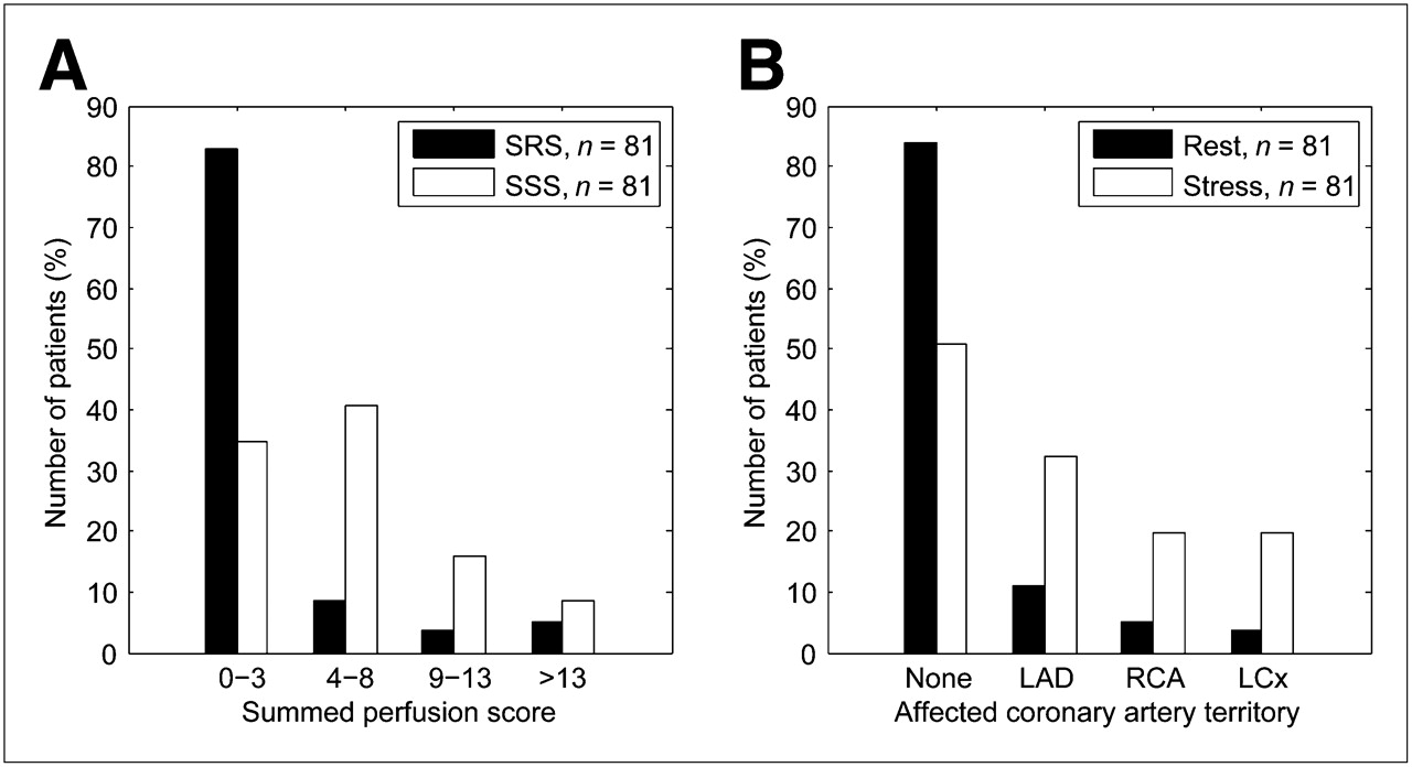
A total of 20 patients (7 women, 13 men; 40 MPS studies) of the study population were selected for training the algorithm (training set), and the remaining 81 patients (30 women, 51 men; 162 MPS studies) were used for prospective validation of the algorithm (test set). The criterion for choosing the training set was the selection of a representative distribution of LVM as determined by MRI. The mean age of the patients in the training set was 62 ± 7 y (range, 51–78 y); in the test set the mean age was 63 ± 12 y (range, 28–82 y). The study population included patients both with and without perfusion defects. The perfusion defect sizes and the defect distribution over the different coronary artery territories in the test set are shown in Figure 1.

(A) Distribution of SRS and SSS in test population. Scores are calculated by QPS, and score of 0 indicates no defect. (B) Distribution of perfusion defects according to coronary artery territories for both rest and stress studies. One patient could be represented in more than 1 group because of presence of multivessel coronary artery disease. LAD = left anterior descending coronary artery; LCx = left circumflex coronary artery; RCA = right coronary artery.
MPS Acquisition and Analysis
MPS images were acquired during rest and stress for each patient. The stress images were acquired after intravenous infusion of adenosine or dobutamine, according to established clinical protocols (98 patients were intravenously infused with adenosine, and 3 patients with dobutamine). All rest and stress images for the same patients were acquired within, at most, 5 d of each other. Only nongated MPS images were used in this study, so that assessment of LVM and perfusion defect size could be performed in the same image set, making it possible to estimate perfusion defect size as percentage of LVM. Patients were injected with 99mTc-tetrofosmin (500–700 MBq) (Amersham Health), depending on their body weight. MPS was performed according to established clinical protocols using a dual-head camera (Vertex; ADAC). The patient was placed supine and imaged in steps of 5.6° using a 64 × 64 matrix, with a typical pixel size of 5 × 5 mm and a slice thickness of 5 mm. Image acquisition time was approximately 15 min. Iterative reconstruction using maximum-likelihood expectation maximization was performed, with a low-resolution Butterworth filter and a cutoff frequency set to 0.5 of Nyquist and an order of 5.0. The full width at half maximum of the point-spread function of the Butterworth filter was 10.6 mm. No attenuation or scatter correction was applied. Finally, short-axis images were reconstructed semiautomatically with manual adjustments, using the program AutoSPECT Plus (Pegasys software, version 5.01; Philips).
The reconstructed MPS images were loaded into QPS (1) (Pegasys software, version 5.01; Philips). The left ventricle and the perfusion defects were automatically segmented without manual corrections. The data were processed by 2 experienced technicians (15 and 28 y of experience), and the quality of the contours of the left ventricle were formally judged by 2 experienced researchers and clinicians (8 and 14 y of experience). Thereafter, LVM, the perfusion defect sizes, and the distributions of the defects over the different coronary artery territories were quantified (1). The left ventricle was divided into 20 segments by the program, and uptake in each segment was graded on a 4-point scale ranging from 0 (normal) to 3 (maximum defect severity). The segments were assigned to 1 of the 3 vascular territories: left anterior descending coronary artery, right coronary artery, and left circumflex coronary artery (Fig. 1). The summed rest score (SRS) and summed stress score (SSS) were calculated by adding the scores in all segments (Fig. 1). The presence of a perfusion defect in a given vascular territory was defined by a score greater than or equal to 4 in that territory.
Extracardiac activity in the MPS images was defined as a region of high count intensity less than 1 wall thickness away from the left ventricular (LV) wall. All images, in both the training set and the test set, were visually assessed to determine the presence of extracardiac activity. An example of an image stack with extracardiac activity is shown in Supplemental Figure 1 (supplemental material is available online only at http://jnm.snmjournals.org).
MRI Acquisition and Analysis
MR images were acquired on the same day as rest MPS images. Image data were acquired in both short-axis and long-axis projections with a 1.5 T scanner (Intera; Philips). Short-axis imaging covering the entire left ventricle was undertaken using a balanced steady-state free precession sequence that was retrospectively triggered to the electrocardiogram. Typical imaging parameters were repetition time/echo time, 2.9/1.5 ms; flip angle, 60°; time frames per cardiac cycle, 30; pixel resolution, 1.4 × 1.4 mm; slice thickness, 8 mm; and slice gap, 0 mm.
All image analysis was performed using the freely available software Segment (version 1.699; http://segment.heiberg.se). LVM by MRI was measured manually in contiguous short-axis images. The endocardium and epicardium of the left ventricle were manually traced in each image slice in both end diastole and end systole. End diastole was defined as the first time frame, and end systole as the time frame with the smallest ventricular cavity. The most basal and apical slices were defined by comparison with the long-axis images, using established methods (5). Papillary muscles that were not contiguous with the myocardial wall were excluded. LVM was calculated as the area between the epicardial and endocardial border multiplied by the slice thickness and a density of 1.05 g/cm3. LVM was defined as the mean value of LVM in end diastole and end systole. Tracings were considered acceptable when the difference in LVM between end diastole and end systole was less than or equal to 2% of their mean. To determine intra- and interobserver variability, MR images from 10 randomly chosen patients from the test set were delineated by a second observer and redelineated by the first observer more than 1 mo later.
MPS Segmentation Algorithm
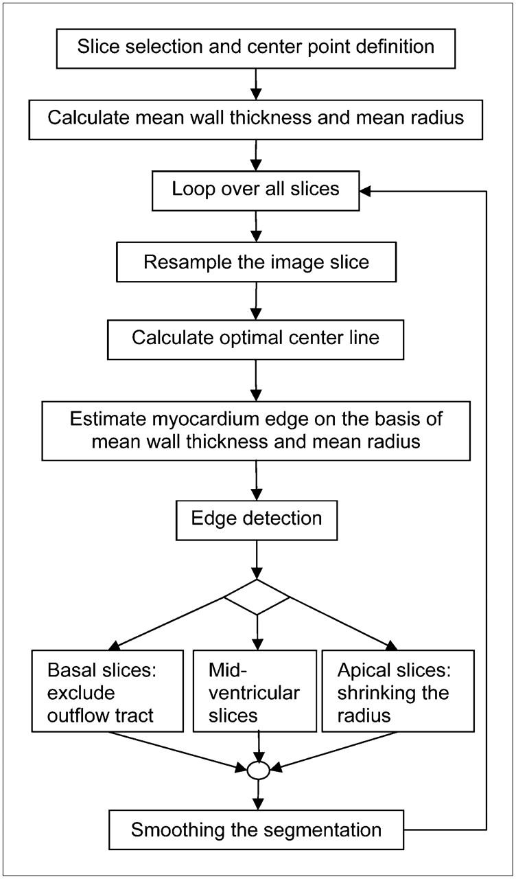
The segmentation algorithm for MPS developed in this study is fully automated and implemented in the freely available research software Segment (http://segment.heiberg.se). In cases in which the algorithm might fail, the user can perform manual corrections. However, no manual corrections were performed in this study. The flow scheme for the segmentation algorithm proposed in this study is illustrated in Figure 2. The segmentation process was started by automatic detection of the most basal slice, the most apical slice, the center point of the left ventricle, mean wall thickness, and mean radius of the myocardium. The thresholds used in the segmentation process were all determined in the training set by 1 of the following 4 processes: The measure by MPS was defined so that the difference in LV length between MPS and MR was minimized (denoted OPT length), the dimension of the left ventricle was measured by MRI (denoted MR), the measure by MPS was defined so that the difference in LVM between MPS and MRI was minimized (denoted OPT LVM), and the optimal measure was visually estimated from the MPS images (denoted MPS). Because the majority of the thresholds were defined using the MR images, the segmentation method will potentially work for other tracers and other MPS acquisition protocols.

Flow scheme for proposed segmentation algorithm.
Identification of Most Basal and Apical Slices.
The most basal and apical slices were identified within a rectangular region of interest 20% smaller in length and width than the original image and centered in the image. This region was chosen to minimize the influence of extracardiac activity. The most basal slice in the short-axis image stack was defined as the first slice apical to that in which pixels exceeding 30% (OPT length) of the maximal intensity occupied an area exceeding 75 mm2 (OPT length). The most apical slice was defined as the first slice in which pixels exceeding 40% (OPT length) of the maximal intensity occupied an area exceeding 200 mm2 (OPT length). To determine if the patient had an apical defect, the mean radius of the mid-mural line of the myocardium was calculated (Appendix) in the most apical slice after resampling of the image slice, as illustrated in Figure 3. If this radius exceeded 10% (MR) of the mean radius in the mid-ventricular slice, then the patient was determined to have an apical defect. If so, the mean radius was extrapolated in the apical direction, and the new most apical slice was defined as the slice with a mean radius closest to 10% of the mean radius in the mid-ventricular slice.
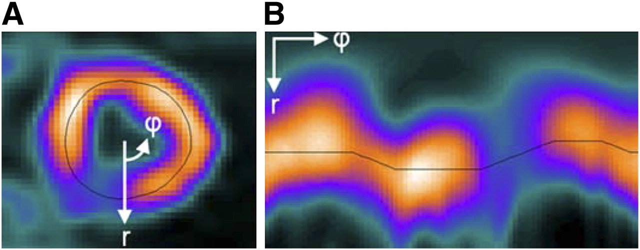
Illustration of resampling process. One radial profile in original image slice (A) is sampled every 4.5°, which results in 80 columns in resampled image (B). Black line in images illustrates estimated mid-mural line through center of myocardium. r = radial direction; φ = circular direction.
Identification of Center Point.
The center point of the left ventricle was calculated in the mid-ventricular short-axis slices (the slices encompassing the mid-ventricular 65% (MR) of the left ventricle) by applying an optimization algorithm to each slice. The start value for the optimization was the pixel in the middle of the image slice. From this center point, a profile of the intensity values in 40 radial directions was calculated. The 2 maximum points corresponding to the mid-mural part of the myocardial wall in each profile were identified, and the middle between these 2 points was the center point for that profile. By taking the mean of these center points over all profiles, a new center point in that image slice was calculated. The algorithm was terminated when the center-point movement was smaller than 0.5 mm or the number of iterations exceeded 10. When the center point was calculated in all mid-ventricular slices, a straight line from base to apex, adjusted to these center points in a least-squares sense, defined the center points of the left ventricle for all short-axis slices. Hereby, the line was adjusted to the correct angle through the slices regardless of errors in the short-axis reconstruction.
Determination of Wall Thickness.
An individual mean wall thickness and mean radius were calculated from the image slice with the highest total intensity. This image slice was first resampled, as illustrated in Figure 3, and then an optimization algorithm (Appendix) identified the mid-mural line in the LV wall. The mean radius was defined as the mean of the distances between the center point of the left ventricle and the points on the mid-mural line. The endo- and epicardial edges were defined as 2 lines on different sides of the mid-mural line in the radial direction. To define these lines, the maximal intensity within 7 mm (MR) around the mid-mural line in each radial direction was identified. The restriction on the region for estimation of the maximal intensity prevents extracardiac activity from affecting the value. The lines were then determined as the pixel with intensity corresponding to 85% (OPT LVM) of the maximal intensity. The mean wall thickness was then calculated as the mean of all distances between the 2 edges that were between 4 and 14 mm (MR).
Detection of Endo- and Epicardium.
The edge detection of the myocardium in the left ventricle was started in the most basal slice. Each slice was first resampled, as illustrated in Figure 3, and then an optimization algorithm based on Dijkstra's algorithm (Appendix) identified the mid-mural line. This line was then forced to be within 70%−130% (MR) of the previously calculated individual mean radius to prevent the mid-mural line from migrating out into the right ventricle or extracardiac activity or from getting too close to the LV center point.
To find the myocardial edges, the previously calculated mean wall thickness was used. The endocardium and epicardium were first estimated by adding to and subtracting from the mid-mural line half the mean wall thickness. The maximal intensity within 7 mm (MR) around the mid-mural line in each radial direction was determined, and the program then performed a search within 4 pixels (corresponding to approximately 3.2 mm in the resampled image) around these myocardial edges. The pixels where the signal intensity was as close as possible to the threshold, defined as 85% (OPT LVM) of the maximal intensity in the radial direction, were then identified.
Identification of LV Outflow Tract.
In the basal slices, defined as the first 20% (MR) of the selected slices, a search for the LV outflow tract was performed. This outflow tract was defined as a continuous region of the myocardium that was centered in the middle of the septum and had a mean intensity in the radial direction below 30% (MPS) of the maximum intensity in the myocardium. The outflow tract was then set to have no myocardial wall thickness.
Processing of Apical Slices.
The last 15% (MR) of the selected slices were defined as the apical slices. In these slices, the radius of the myocardium was set to diminish successively. An edge detection within 2 pixels, as described earlier, was then performed for both the endocardium and the epicardium in the apical slices.
Finally, the segmentation, represented as 1 endocardial surface and 1 epicardial surface, was smoothed along the respective surfaces in circumferential and longitudinal directions with a 5 × 5 Gaussian kernel.
Validation
To validate the proposed segmentation approach, the algorithm was applied to the test set of 81 patients (162 MPS studies). The LVM in the MPS images was then compared with the LVM from manually segmented MR images for both LVM according to the new method and LVM as determined by QPS. The endo- and epicardial delineations obtained with the new method were also visually inspected and classified as either reasonable or unreasonable.
Sources of Error.
To further evaluate the segmentation process, 5 different parameters were tested for correlation with the error in LVM between MPS and MRI. The 5 parameters were heart rate, summed rest or stress perfusion score (SRS and SSS), LV radius by MRI, LV length by MRI, and wall thickness by MRI. The LV length by MRI was measured as the distance between the most basal and apical slices in the segmentation in end diastole. The LV radius in MRI was defined as the average distance between the mid-mural line of the myocardium and the LV center point in the mid-ventricular short-axis slices.
The wall-thickness estimation in the segmentation process was evaluated by analyzing the intensity over the myocardium in the radial direction in the MPS images for 4 groups of test patients. These groups were divided according to the wall thickness determined by MRI: 6–9 mm (25 patients, 50 MPS studies), 9–10 mm (20 patients, 40 MPS studies), 10–11 mm (20 patients, 40 MPS studies), and 11–13 mm (16 patients, 32 MPS studies).
Statistical Analysis
Values are presented as mean ± SD. Pearson linear regression analysis was performed to calculate the relationship between 2 variables. A P value of less than 0.05 was considered statistically significant. The error in LVM was calculated as ([LVM by MPS] − [LVM by MRI])/(LVM by MRI). Inter- and intraobserver variabilities were calculated as the mean ± SD of the difference between observations. The coefficient of variance (CV) was calculated as the SD of the difference between observations divided by their mean. Differences in mean difference were analyzed by the t test, and differences in SD were analyzed by the F test.
RESULTS
Figure 4 shows segmentations performed in 1 patient with high discrepancies in LVM between the new method and QPS. The automatic segmentation algorithm was deemed reasonable in 100% (162/162) of the cases, which means that no manual correction was performed, and in no case was the segmentation deemed unreasonable. The contours of the left ventricle, determined by QPS, were in all cases assessed by the 2 experienced researchers and clinicians to fulfil clinical and research standards. The segmentation algorithm took about 10 s to perform on a standard personal computer (3-GHz processor, 1 GB RAM).
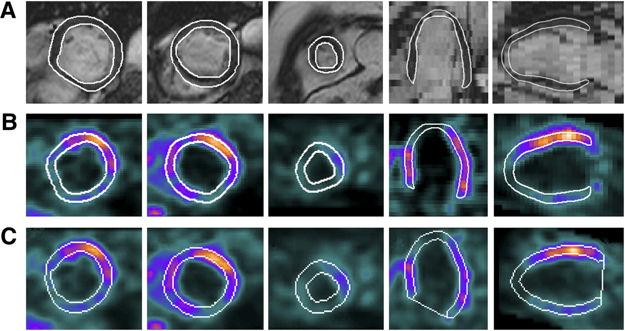
Illustration of segmentation of LVM in 1 patient with high discrepancies between new method and QPS. (A) MR images with manual LV segmentation. (B) MPS images with segmentation performed by new method. (C) MPS images with segmentation performed by QPS. LV segmentation is illustrated as white lines in all images. LVM quantified by MRI was 171 g, by new method 176 g, and by QPS 202 g. New method, compared with LVM by MRI, overestimated LVM by 3% LVM and QPS by 24% LVM.
Interobserver variability was 8% ± 8% LVM and CV was 6%, whereas intraobserver variability was 1% ± 4% LVM and CV was 3%.
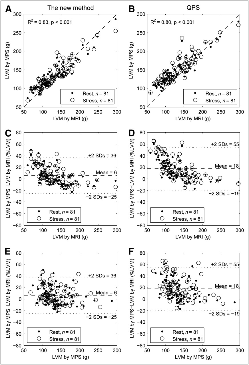
The results from the LVM comparison are shown in Table 1. The mean difference ± SD in LVM between MPS and MRI was lower for the new method than for QPS for both mean difference (P < 0.001) and SD (P = 0.015). Figure 5 shows the relationship between LVM by MPS (both rest and stress) and by MRI, using both the new method and QPS. Linear regression analysis between rest MPS and stress MPS (interstudy variability) resulted in a mean difference of 0% ± 6% (R2 = 0.95) for the new method and 2% ± 6% (R2 = 0.95) for QPS. The CV between rest MPS and stress MPS was 6% for both the new method and QPS.

(A) Relationship between LVM measured by MPS, segmented by new method, and by MRI. Dashed line is line of identity. (B) Relationship between LVM measured by MPS, segmented by QPS, and by MRI. Dashed line is line of identity. (C) Relationship between error in LVM, for new method, and LVM by MRI. (D) Relationship between error in LVM, for QPS, and LVM by MRI. (E) Relationship between error in LVM, for new method, and LVM by MPS. (F) Relationship between error in LVM, for QPS, and LVM by MPS. Note in C and D trend of decreasing error and variability with increasing LVM by MRI. This trend is not present in E and F when LVM by MPS is on horizontal axis. This absence of trend illustrates that LVM from MPS alone cannot be used to adjust algorithm to improve agreement between MPS and MRI.
Results for LVM Comparison Using New Segmentation Algorithm and QPS
Extracardiac activity was present in 3 of 40 studies in the training set (8%) and in 18 of 162 studies in the test set (11%). The difference in LVM between MPS and MRI for the new method was 6% ± 15% LVM when all cases in the test set were included and 5% ± 15% LVM when the cases with extracardiac activity were excluded. For QPS, the results were 18% ± 19% LVM and 17% ± 18% LVM, respectively. Both mean difference (P < 0.001) and SD (P = 0.018) were still, when the cases with extracardiac activity were excluded, significantly lower for the new method than for QPS.
Figure 5C shows a trend of overestimation of LVM for small hearts (low LVM) and underestimation of LVM for big hearts (high LVM). To analyze the reason for this over- and underestimation, the correlation of 5 different parameters with the error in LVM were analyzed. The result from the linear regression analysis of these parameters is shown in Table 2. The parameter with the highest correlation with the error in LVM was myocardial wall thickness by MRI. Supplemental Figure 2 shows overestimation of LVM in hearts with thin myocardium and underestimation in hearts with thick myocardium by both the new method and QPS. Supplemental Figure 3 illustrates the intensity in the radial direction over the myocardium in the MPS images for hearts with different myocardial wall thicknesses by MRI.
Results from Linear Regression Analysis of 5 Parameters and Error Between Determining LVM by MPS and by MRI
DISCUSSION
The major finding of this study is that the new LVM segmentation method for MPS shows a good agreement with MRI. The study also shows that accurate estimation of wall thickness is the main source of error in the segmentation process. When comparing LVM between MPS and MRI, the new method has both significantly lower bias and significantly lower variability than does the commercially available program QPS. Thus, the new method is more accurate and more precise at estimating LVM than is QPS. The R2 value for the correlation between LVM by MPS and LVM by MRI was not statistically different between the 2 algorithms, 0.83 (new method) and 0.80 (QPS) in the current study. This finding is in broad agreement with results from other studies with R2 values of 0.83 (3) and 0.79 (2). Notably, methods with similar R2 values do not necessarily have similar bias and variability. It has been suggested that bias and variability are more appropriate than an R2 value when comparing 2 measures (6).
The interstudy reproducibility for quantifying LVM between rest and stress was good for both the new method and QPS. Our results showed a mean difference lower than, and a variability similar to, previous reports of interstudy variability of rest/stress LVM by MPS (10% ± 5% (7) and 6% ± 7% (8)). Both the intra- and the interobserver variabilities were low for the manual delineation of LVM by MRI. These results are similar to those found in prior studies (9), indicating that MRI is a robust reference standard in the current study.
The good agreement between the automatically segmented MPS and manually segmented MRI in determining LVM makes the former method attractive for estimating the size of the perfusion defect when it is expressed as the percentage of the left ventricle. Furthermore, minimizing errors in LV segmentation is necessary for minimizing errors in the segmentation of the perfusion defect size. These results have been achieved in a test population with a clinically relevant distribution of defect sizes and affected coronary artery territories. Furthermore, all 162 of 162 image sets in this study were segmented without manual corrections. This makes the proposed method appropriate for clinical use, a setting in which speed, reproducibility, and ease of use are important.
Several previous studies have compared LV volumes and ejection fraction measured by gated MPS and MRI (10–13). However, only 2 studies have specifically compared LVM measured by MPS and MRI.
Two challenges with LV segmentation in MPS images are identifying the most basal slice and avoiding errors due to extracardiac activity. The thresholds used for identifying the most basal slice are the result of optimization in the training set, which included both patients with and patients without basal defects. The identification of the most basal slice was, hereby, successful in both categories of patients. The restrictions in the mid-mural line and wall-thickness estimation prevent the LV segmentation from migrating out into extracardiac activity and make the new method successful in separating the left ventricle from the extracardiac activity in all patients (Supplemental Fig. 1). The performance of the new method and QPS in the absence of cases with extracardiac activity yielded results that were essentially unchanged. Both the mean difference and the SD were still significantly lower for the new method than for QPS when the cases with extracardiac activity were excluded.
Sources of Error in the Segmentation Process
The overestimation of LVM in small hearts (low LVM) and underestimation in big hearts (high LVM), which was found in the current study, is in agreement with an earlier study (3). Similar to a previous study (14), our results showed that heart rate did not correlate with the error in LVM; thus, the segmentation works equally well independent of how fast the heart moves over time. The second parameter that did not correlate with the error in LVM was the summed perfusion score; thus, the segmentation algorithm worked equally well regardless of the presence, extent, and severity of perfusion defects. Furthermore, the LV length and radius correlated poorly with error in LVM. This finding implies that it is neither slice selection nor calculation of the mid-mural line that is the major source of error in LVM segmentation. The parameter that by far had the highest correlation with error in LVM was wall thickness by MRI, both for the new method and for QPS, indicating that estimation of wall thickness is the main source for error in segmentation of LVM by MPS. Our results showed that wall thickness was overestimated in hearts with thin myocardium and underestimated in hearts with thick myocardium, because the intensity curves in the radial direction over the myocardium were highly similar, independent of true wall thickness (Supplemental Fig. 3). This result shows the difficulty in separating these groups from each other with regard to wall thickness. The similar intensity curves are probably mostly due to the limited spatial resolution in the MPS images, resulting in blurring due to the partial-volume effect. The limited spatial resolution is therefore a fundamental limitation for highly accurate quantification of LVM in MPS. The effects of limited spatial resolution are a well-known problem in quantitative analysis of MPS images (15).
Compensation for Limited Spatial Resolution
To achieve an even more reliable segmentation than the resulting segmentation in this study, estimation of the wall thickness needs to improve. As shown in this study, this improvement is not possible with the spatial resolution of current MPS, because all hearts appear to have approximately the same wall thickness, as seen by the myocardial wall intensity profiles (Supplemental Fig. 3). Notably, these in vivo results agree with a previous phantom study (16).
However, some studies have attempted to use different correction methods to overcome the problems caused by limited spatial resolution. All these studies show promising results with their correction methods but have different limitations. One study (17) requires the acquisition of a blood-pool image of the heart to calculate the correction coefficient. Correction methods that use only information in the original MPS image have been proposed by Galt et al. (18) and El Fakhri et al. (19). The correction method proposed by Galt et al. was tested on phantoms assuming equal maximum intensity around the myocardium. This correction method could therefore cause problems in patients with perfusion defects. In the study by El Fakhri et al., the correction method was based on an assumption of a 10-mm-thick myocardium. This correction method will, therefore, not distinguish hearts with thin myocardium from hearts with thick myocardium. Thus, neither of these correction methods was attempted in the current study, nor would they be expected to offer any substantial improvement in accuracy or precision compared with the proposed new method.
As discussed by King et al. (20), the threshold to identify a correct edge is dependent on the diameter of the source. The smaller the diameter of the source is, the higher a threshold is needed, as was verified by our study, in which the thinnest myocardium was overestimated and a higher threshold needed to more accurately estimate the edge of the myocardium. Hence, the threshold in the segmentation algorithm needs to change according to the wall thickness of the heart. The threshold can be changed by taking information from, for example, an MR image, but such a procedure is not practical in the clinical setting.
Study Limitations
A limitation when comparing LVM from MPS with LVM from MRI is that the papillary muscles are visible in the MR images but not in the MPS images. Thus, the muscles can be excluded from the segmentation in the MR images. In MPS, the papillary muscles are incorporated in the wall because of the limited spatial resolution.
CONCLUSION
This study presents and validates an automatic method to segment the left ventricle in MPS images. The method shows good agreement in comparisons of the LVM by MPS with the LVM by MRI, and quantification of LVM is important for estimating the size of a perfusion defect as a percentage of the left ventricle. Both the mean difference and the SD in LVM between MPS and MRI were significantly lower for the new method than for a commercially available algorithm. The main source of error in the segmentation process is the estimation of the myocardial wall thickness, and this source of error is currently difficult to overcome using information found only in the MPS images.
APPENDIX
Estimation of the Mid-Mural Line of the Myocardium
To find the mid-mural line of the myocardium, an optimization algorithm was applied to the resampled short-axis slice. The mid-mural line was defined as the line through the points with highest signal intensity. The algorithm was based on Dijkstra's algorithm for finding a global optimal minimal cost path between a numbers of nodes. The cost function was defined so that high intensity and a horizontal line give low cost, and low intensity and high slope on the curve give a higher cost. In Figure 3, an example of this mid-mural line is illustrated as a black line through the myocardium.
The resampled image was taken as input to the optimization algorithm together with rigidity and elasticity parameters. g denotes the intensity value from the resampled image, f denotes the active contour (here the radius of the myocardium), α the elasticity, and β the rigidity. The optimization problem to solve was  .
.
To solve this equation, f was restricted to a discrete function y(x), and the optimization problem could then be approximated by (21):
 (Eq. 1A)where L is the number of columns in the discrete grid, and M is the number of rows in the discrete grid. Eimage represents the total intensity along the mid-mural line, which should be maximized (thus the minus in the optimization), and Eint represents the slope of the line, which should be minimized.
The rigidity and elasticity parameters were determined to minimize the risk for the curve to migrate out into the right ventricle but still be flexible enough to follow the myocardial shape. The values used in the test set, optimized in the training set, were α = 0.015 and β = 0.015.
Acknowledgments
We thank technicians Ann-Helen Arvidsson and Christel Carlander for invaluable help with data acquisition. Funding for this project comes in part from the Swedish Heart Lung Foundation, Sweden; Lund University Faculty of Medicine, Lund, Sweden; the Swedish Research Council, Sweden; and the Region of Scania, Sweden.
Footnotes
-
COPYRIGHT © 2009 by the Society of Nuclear Medicine, Inc.
References
- Received for publication August 21, 2008.
- Accepted for publication October 21, 2008.


