


Abstract
Detecting perfusion interhemispheric asymmetry in neurologic nuclear medicine imaging is an interesting approach to epilepsy. Methods: This study compared 4 methods that detect interhemispheric asymmetries of brain perfusion in SPECT. The first (M1) was conventional side-by-side expert-based visual interpretation of SPECT. The second (M2) was visual interpretation assisted by an interhemispheric difference (IHD) volume. The last 2 were automatic methods: unsupervised analysis using volumes of interest (M3) and unsupervised analysis of the IHD volume (M4). Use of these methods to detect possible perfusion asymmetry was compared on 60 simulated SPECT datasets by controlling the presence and location of asymmetries. From the detection results, localization receiver operating characteristic curves were generated and areas under curves were estimated and compared. Finally, the methods were applied to analyze interictal SPECT datasets to localize the epileptogenic focus in temporal lobe epilepsies. Results: This study showed an improvement in asymmetry detection on SPECT images with the methods using IHD volume (M2 and M4), in comparison with the other methods (M1 and M3). However, the most useful method for analyzing clinical SPECT datasets appeared to be visual inspection assisted by the IHD volume, since the automatic method using the IHD volume was less specific. Conclusion: The use of quantitative methods can improve performance in detection of perfusion asymmetry over visual inspection alone.
The investigation of intractable partial epilepsy is based on a combination of video electroencephalography (e.g., clinical observation correlated with electroencephalography) and imaging findings. The efficiency of 99mTc-hexamethylpropyleneamine oxime (HMPAO) and 99mTc-ethylcysteinate dimer (ECD) SPECT has largely been demonstrated for detecting perfusion abnormalities and helping to identify the epileptogenic focus (1).
In clinical routine, the analysis of brain SPECT images is often limited to qualitative side-by-side visual inspection. Such an interpretation is user dependent and subjective. Quantification might thus improve diagnostic accuracy.
The relationship between blood flow and 99mTc-HMPAO or 99mTc-ECD SPECT brain uptake is nonlinear because of a saturation phenomenon; absolute measurement of regional cerebral blood flow from HMPAO/ECD SPECT scans is therefore not feasible. Thus, relative quantification methods are often proposed. Methods based on regions of interest or volumes of interest (VOIs) (2–4) are used for either intrascan studies or interscan studies (intra- or intersubjects). The term intrascan refers to an analysis limited to a single scan. The term interscan refers to an analysis involving several scans. Similarly, intrasubject denotes analysis limited to a single subject, whereas intersubject denotes analysis involving datasets obtained from several subjects. Voxel-based methods are used for interscan studies only. In the detection of epileptogenic foci, an intrasubject voxel-based method consists of subtraction of ictal and interictal SPECT scans after they have been coregistered to MRI scans (5,6). Intersubject approaches compare the scans of epileptic subjects with those of a control group (7).
The aim of this study was to compare the performance of 4 methods highlighting intrascan interhemispheric variations in SPECT: conventional side-by-side visual interpretation by an observer (M1), visual interpretation assisted by the interhemispheric difference (IHD) volume (created by the unsupervised voxel neighborhood method (8)) (M2), unsupervised analysis using VOIs (M3), and unsupervised analysis of the IHD volume (M4) (8).
These methods were compared using simulated SPECT datasets including known asymmetries and using clinical SPECT datasets with cerebral blood flow variations difficult to see with the naked eye (interictal SPECT scans of patients with temporal lobe epilepsy).
MATERIALS AND METHODS
Methods of Detecting Interhemispheric Asymmetry in Perfusion
Visual Inspection (M1).
The first method was conventional visual interpretation of SPECT with side-by-side comparison. This analysis was done by 4 observers experienced in image analysis: 2 nuclear medicine physicians, a neurosurgery resident, and a neurologist.
Visual Interpretation Assisted by IHD Volume (M2).
The SPECT dataset and the IHD volume were inspected simultaneously by the observer. The goal of adding IHD volume (8) was to help detect interhemispheric asymmetries in perfusion on brain SPECT scans, using anatomic information available from MRI scans. For this purpose, the IHD volume was computed at the MRI spatial resolution. For each MRI voxel, the anatomically homologous voxel in the contralateral hemisphere was identified. Both homologous voxel coordinates were then mapped into the SPECT volume using SPECT-MRI registration. Neighborhoods were then defined around each SPECT voxel and compared. A relative difference value was thus computed from both neighborhoods and assigned to the MRI voxel to obtain the volume of IHDs.
Approaches based on optimization of statistical similarity measurements have produced accurate SPECT-MRI registration (9). Using realistic simulations of normal and ictal SPECT images, we compared the spatial accuracy of major similarity-based registration methods used for SPECT-MRI registration, namely mutual information (10), normalized mutual information (11), correlation ratio (12), and the criterion of Woods et al. (13). Apart from that criterion, we found similar accuracy for these methods (14). We thus chose to perform rigid SPECT-MRI registration using maximization of mutual information (10).
For every voxel of the MRI volume, the voxel that was anatomically homologous in the contralateral hemisphere was identified, using the spatial normalization scheme provided in the Statistical Parametric Mapping (SPM) software package (15). This method computed a nonrigid transformation between the MRI scan of the patient and the T1 template (average of 152 normal MRI scans after realignment with the Talairach system), which had been modified to be symmetric. Using this transformation, the voxel corresponding to each point of the patient’s MRI scan was identified in the template. Because the template was modified to be symmetric, the homologous voxel in the contralateral hemisphere was obtained by symmetry over the sagittal plane. Using the inverse transformation (calculated from the T1 template to the MRI scan), the coordinates of the homologous voxel in the patient’s MRI scan were determined. The voxel coordinates were then transferred to the already-coregistered SPECT volume to define voxel neighborhoods.
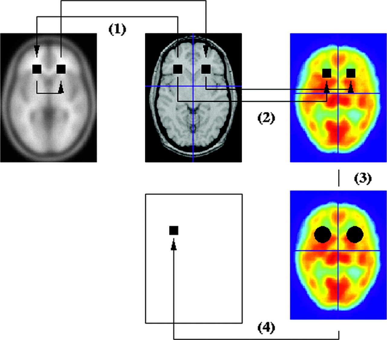
Two symmetric spheric voxel neighborhoods (diameter of 18 mm) containing 33 voxels were defined on SPECT data around the 2 homologous voxels. The empiric means (x1 and x2) of the voxel SPECT intensity values in both neighborhoods were calculated and the normalized difference D, defined by  , was deduced. This result was stored in a volume of differences at the same coordinates as the initial voxel within the MRI volume (Fig. 1). The calculation was repeated for each MRI voxel in a brain mask to fill the IHD volume.

Creation of IHD volume: (1) identification of homologous voxels; (2) transfer of MRI voxel coordinates to SPECT volume (SPECT-MRI registration); (3) definition of voxel neighborhoods; (4) calculation of normalized difference, stored in difference volume at same coordinates as initial voxel within MRI volume.
Automatic VOI-Based Method (M3).
Sixty-three anatomic structures, or VOIs of intra- and extracerebral anatomic structures, have been hand-drawn and labeled by Zubal et al. (16) from a high-resolution 3-dimensional (3D) T1-weighted MRI scan of a healthy subject (124 axial slices; matrix, 256 × 256; voxel size, 1.1 × 1.1 × 1.4 mm). This labeled anthropomorphic model of the head is called the Zubal phantom.
To perform SPECT measurements on the VOIs (Fig. 2), we used the spatial normalization method described by Friston et al. (15) and implemented in the SPM software (SPM99). Both SPECT data and VOIs were spatially normalized to a mean anatomic reference volume, represented by the T1 template provided by SPM, as follows. A nonlinear geometric transformation was estimated to match the 3D T1-weighted MRI scan of the Zubal phantom and, thus, the VOIs on the SPM T1 template. A 2-step approach was used to spatially normalize SPECT data. First, an intermodality-intrapatient rigid registration was performed between the SPECT and MRI data of each patient, by maximization of mutual information. Second, the 3D T1-weighted MRI scan of each subject was spatially normalized to the SPM T1 template, using a nonlinear geometric transformation. These linear and nonlinear geometric transformations were used to resample the SPECT data and the predefined VOIs of the Zubal phantom in the SPM T1 template using trilinear interpolation.

VOI-based method.
For a spatially normalized predefined VOI of the Zubal phantom and spatially normalized SPECT data, we estimated the mean intensity of the SPECT voxels (x̄) within the considered VOI. For each pair of lateralized VOIs, the empiric means (x1 and x2) were calculated and the normalized difference D was deduced  .
.
Automatic IHD Volume-Based Method (M4).
The unsupervised analysis of the IHD volume (detailed in the paragraph describing M2) consisted of studying the voxel of the IHD volume with maximum intensity. VOIs are used to give the anatomic location of this voxel. Because the VOIs are in the T1 template anatomic reference, IHD volume was also spatially normalized to this T1 template.
Method of Evaluation
Simulated Datasets.
To determine and compare the ability of the 4 methods to detect perfusion asymmetry zones of various sizes and amplitudes, we simulated 40 SPECT datasets including perfusion asymmetries of known size and amplitude. In the same way, 20 SPECT datasets without perfusion asymmetry were simulated.
Realistic analytic SPECT simulations require an activity map representing the 3D spatial distribution of the radiotracer and the corresponding attenuation map describing the attenuation properties of the body. The attenuation map was obtained by assigning a tissue type to each VOI of the Zubal phantom (conjunctive tissue, water, brain, bone, muscle, fat, and blood). Each tissue type was assigned an attenuation coefficient μ at the 140-keV energy emission of 99mTc: connective tissue (μ = 0.1781 cm−1), water (μ = 0.1508 cm−1), brain (μ = 0.1551 cm−1), bone (μ = 0.3222 cm−1), muscle (μ = 0.1553 cm−1), fat (μ = 0.1394 cm−1), and blood (μ = 0.1585 cm−1).
A theoretic model of brain perfusion, mimicking mean normal perfusion, was established from real SPECT data (27 healthy subjects) to construct the theoretic activity map (17). This construction involved spatial transformation of these SPECT data into a mean anatomic reference volume and quantitative measurements using the anatomic entity masks extracted from the labeled MRI scan, after spatial normalization.
From the theoretic activity map, we introduced single zones of various sizes and intensities of perfusion asymmetry in the gray matter of the frontal, occipital, parietal, or temporal lobes. The asymmetric zones were spheres with a radius of 5, 10, 15, or 20 mm, defined on the activity map. So that realistic perfusion abnormalities would be modeled, only gray matter voxel values were increased or decreased (baseline activity ± 10%, 20%, 30%, or 40%). With 4 possible sizes (from spheres with a radius of 5, 10, 15, or 20 mm), 8 possible intensities (baseline activity ± 10%, 20%, 30%, or 40%), and 4 possible localizations (frontal, occipital, parietal, or temporal lobes), 128 datasets including a single perfusion asymmetry could be simulated. The 40 datasets used in this study were randomly selected from these 128 possible datasets.
These attenuation and activity maps were used to simulate SPECT projections, taking into account nonuniform attenuation (64 projections in a 128 × 128 matrix over 360°; RecLBL software package [Lawrence Berkeley Laboratory] (18)). Collimator and detector responses were simulated using a gaussian filter of 8 mm in full width at half maximum (FWHM). Poisson noise was also included on these projections. Images were reconstructed using filtered backprojection with a Nyquist-frequency-cutoff ramp filter, and the reconstructed images were postprocessed using a 3D gaussian filter with a FWHM of 8.8 mm, leading to a resolution of 12 mm. Through construction, the simulated SPECT data were perfectly aligned with the Zubal phantom MRI data.
Data Analysis.
For visual inspection, 4 clinicians analyzed 60 simulated SPECT datasets either with or without perfusion asymmetry in the temporal, frontal, parietal, or occipital lobe. They were unaware of the patients’ clinical data. The reading was performed in 2 independent steps: with and without the assistance of the IHD volume. The clinicians indicated whether the image showed asymmetry using a certainty scale from 1 to 5 (1, definitely no; 2, probably no; 3, possibly yes; 4, probably yes; and 5, definitely yes). In addition, for scores from 3 to 5, the readers indicated the location of the asymmetry (temporal, frontal, parietal, or occipital lobe).
The unsupervised analysis of the IHD volume consisted of studying the voxel of the IHD volume with the maximum D intensity. This voxel could be in a lobe (temporal, frontal, parietal, or occipital) or elsewhere in the brain. For the VOI-based method, the normalized difference D was computed for lateralized frontal, occipital, parietal, and temporal lobe VOIs. Only the VOI with the highest D value was studied. For these 2 automatic methods, 4 cutoff values were applied to D to obtain values distributed along the 5 certainty levels, as was the case for the clinicians’ answers for M1 and M2.
For each score used as a threshold and for each volume, the detected abnormality could be compared with the known asymmetry. Sensitivity (defined as the percentage of simulated datasets for which asymmetries were properly detected and localized) and specificity (defined as the percentage of simulated datasets without asymmetry for which no asymmetry was detected) were determined.
Method Comparison.
The comparisons between the different methods were assessed using localization receiver operating characteristic (LROC) curves (19). LROC curves were deduced by plotting the true-positive rate (or sensitivity) against the false-positive rate (1 − specificity) for the different thresholds. The area under LROC curves (AUC) was used as an index characterizing the detection performance of the methods. The LROC curves and AUC values obtained for the 4 methods were deduced and compared.
Clinical Application
Patients and Data Acquisition.
Interictal scans of 18 patients (8 women and 10 men; age range, 14–44 y; mean, 25 y) with temporal lobe epilepsy (right temporal lobe epilepsy in 8 patients and left temporal lobe epilepsy in 10) were included in this study. Four patients had a lesional area, and 4 underwent stereo electroencephalography. The duration of epilepsy ranged from 2 to 37 y (mean, 15.6 y). Because all patients underwent a successful resection (seizure-free for at least 2 y after the surgery), the area of resection was assumed to include the epileptogenic focus.
For these 18 patients with temporal lobe epilepsy, interictal SPECT images were acquired with a double-head DST-XL imager (General Electric Medical Systems) equipped with fanbeam ultra-high-resolution collimators (13 patients) or ultra-high-resolution parallel collimators (5 patients). The radiotracer (740 MBq) was 99mTc-HMPAO (3 patients) or 99mTc-ECD (15 patients). Sixty-four projections over 360° (128 × 128 matrix for 15 patients, 64 × 64 matrix for 3 patients; pixel sizes of 4.51 mm for 13 patients, 3.39 mm for 2 patients, and 6.78 mm for 3 patients) were acquired. T1-weighted 3D MRI was also performed with a 1.5-T Signa machine (General Electric Medical Systems): 124 sagittal 256 × 256 slices, 0.9375 × 0.9375 × 1.3 mm voxels, and a spoiled gradient echo sequence (field of view = 24 cm, α = 30°, echo time = 3 ms, repetition time = 33 ms).
SPECT data were reconstructed using filtered backprojection with a ramp filter (Nyquist-frequency cutoff). The reconstructed data were postprocessed with an 8-mm FWHM 3D gaussian filter. The acquisition of linear sources using the clinical acquisition and reconstruction protocols yielded a spatial resolution of 12.2-mm FWHM in the reconstructed images. Assuming uniform attenuation in the head, we performed first-order Chang attenuation correction (20).
Data Analysis.
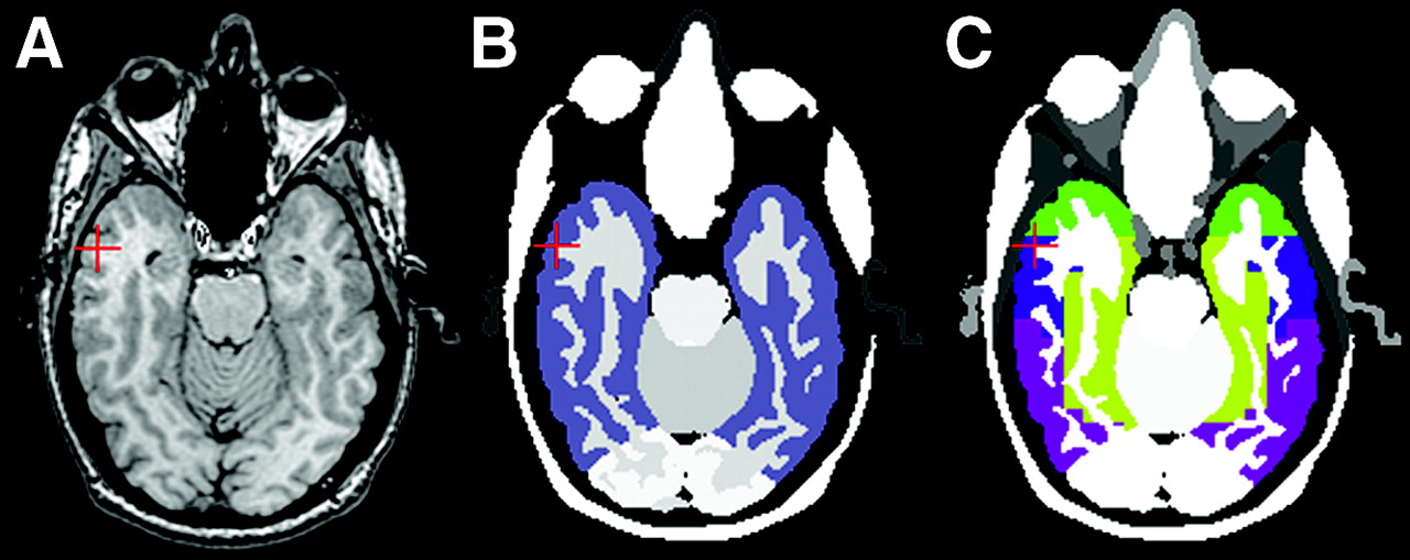
First, the 4 analysis methods were used to detect potential perfusion asymmetry in the temporal lobes of patients (laterality study). Second, these methods were used to localize potential hypoperfusion more precisely in the different regions of the temporal lobe (inner, outer, or polar; Fig. 3) that had undergone a corticectomy (localization study).

(A) Axial slice of temporal VOIs from MRI data. (B) VOI including entire temporal lobe (in purple). (C) Inner (light green), outer (blue), polar (bright green), and posterior (purple) temporal regions.
For M1 and M2, 2 observers (observers 1 and 2 of the previous study) analyzed the color SPECT data and IHD volume (for M2) merged with the MRI data. For the laterality study, they indicated whether hypoperfusion was present in the temporal lobe and, when applicable, the hemisphere concerned. For the localization study, they specified whether hypoperfusion was present for each region of the temporal lobe (inner, outer, or polar). The degree of concordance between the 2 observers could be measured using Cohen’s κ-coefficient, using 2 categories defined as “observer in agreement with surgery” and “observer not in agreement with surgery,” and showed that use of the IHD volume led to an increase in κ from 0.34 (visual inspection) to 0.769 (visual inspection + IHD volume).
For M3, based on the study of VOIs, the IHD was calculated for the VOI including the entire temporal lobe for the laterality study and for the inner, outer, and polar regions for the localization study. If the difference was greater than 5%, the right region was considered to have hypoperfusion; if the value was less than −5%, the left region was considered to have hypoperfusion; and if the value was between −5% and 5%, hypoperfusion was considered undetected. For M4, based on the study of IHD volume, the analysis focused on the highest-intensity voxel (i.e., the highest IHD) in the VOI including the entire temporal lobe for the laterality study and for the inner, outer, and polar temporal regions for the localization study. If the value of this voxel was less than −20% in the right region, this region was considered to have hypoperfusion; if the value was less than −20% in the left region, this region was considered to have hypoperfusion; and if the value was greater than −20%, hypoperfusion was considered undetected. For M3 and M4, the threshold values (5% and 20%, respectively) were chosen experimentally to give the highest possible sum of sensitivity and specificity.
RESULTS
Evaluation of Simulated SPECT Data
For 3 of the 4 observers (observers 1, 2, and 4), the values of the areas under the LROC curves (Table 1) were higher with visual inspection assisted by IHD volume than with visual inspection alone. According to the obtained values of the AUC (from the highest to the lowest), the methods from the most to the least effective were visual inspection assisted by IHD volume (average AUC, 0.62), automatic inspection of the IHD volume (AUC, 0.58), visual inspection alone (average AUC, 0.55), and automatic inspection based on VOIs (AUC, 0.51).
AUC
Clinical Application
Laterality Study.
We compared the results (presence and laterality of hypoperfusion) with the laterality of the epileptogenic focus as validated by patient recovery after surgery. Table 2 shows these results for the 4 methods and the 2 observers. These results enabled us to define 3 cases: identification of hypoperfusion in the same hemisphere identified at surgery (ipsilateral detection), identification of hypoperfusion in the hemisphere contralateral to that identified at surgery, and no identification of hypoperfusion. We could then calculate the ipsilateral detection fraction (idf), the contralateral detection fraction (cdf), and the no-detection fraction (ndf) for each of the analysis methods, as follows: 
 and
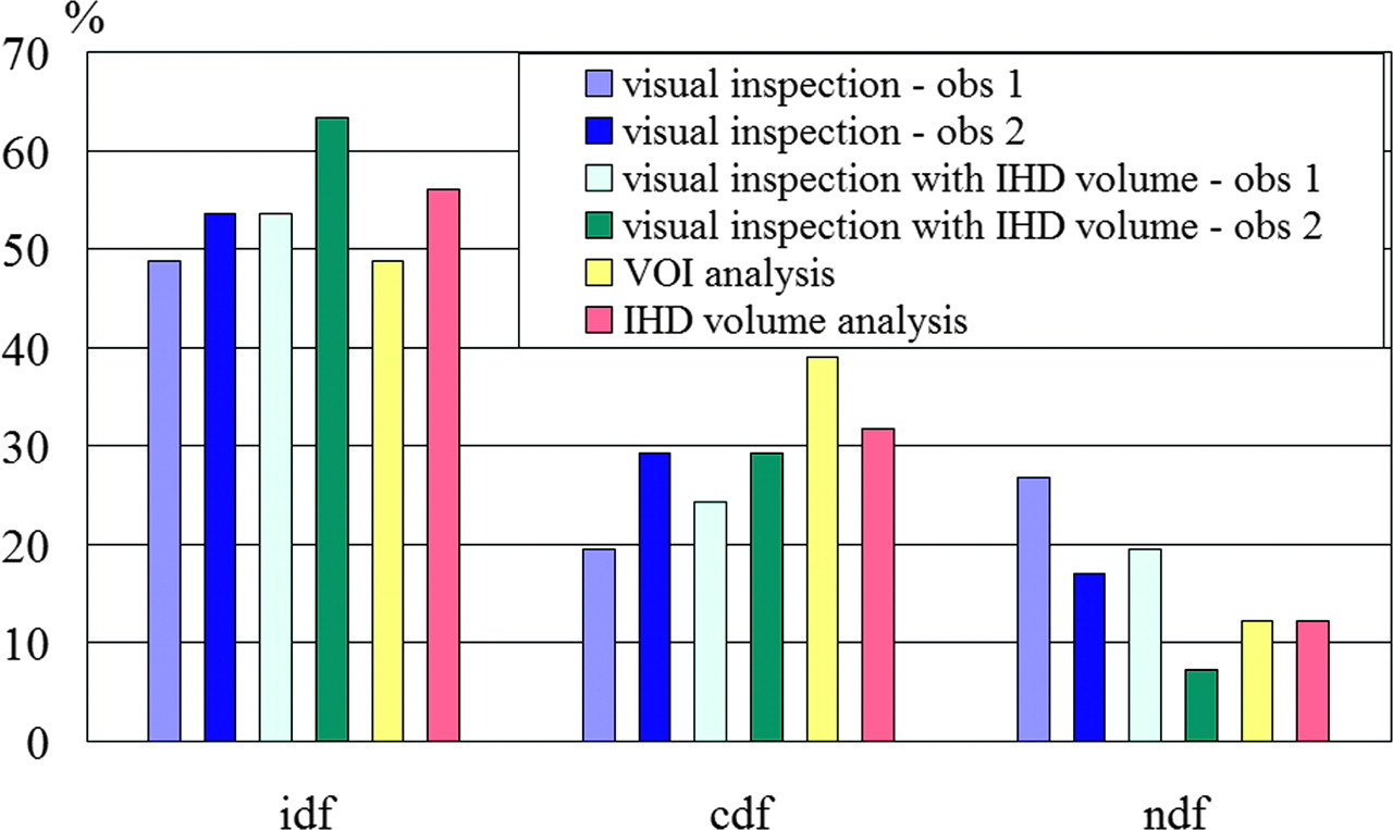
and  These fractions were computed for the 4 methods and the 2 observers (Fig. 4).

Laterality of potential hypoperfusion in temporal lobe: comparison of the 4 detection methods based on clinical data in terms of ipsilateral detection fraction (idf), contralateral detection fraction (cdf), and no detection fraction (ndf). For first 2 methods, involving a human observer, performances are given for the 2 observers (obs 1 and obs 2).
Laterality of Potential Hypoperfusion in Temporal Lobe
Localization Study.
For each patient and temporal region that underwent a corticectomy, we investigated whether hypoperfusion was detected by the different methods. The regions that underwent corticectomy could be either the outer part of the temporal lobe; the inner and the outer parts; or the inner, outer, and polar parts. Thus, for all the data, 41 regions were studied. Figure 5 shows the values of the ipsilateral detection fraction, the contralateral detection fraction, and the no-detection fraction computed for the 41 regions that underwent a corticectomy leading to patient recovery.

Localization of potential hypoperfusion in different parts of temporal lobe: comparison of performance of the 4 detection methods based on clinical data in terms of ipsilateral detection fraction (idf), contralateral detection fraction (cdf), and no detection fraction (ndf). For first 2 methods, involving a human observer, performances are given for the 2 observers.
DISCUSSION
Use of the IHD volume, whether automatic or in addition to visual inspection of SPECT data, would appear relevant. Indeed, the values of the areas under curves obtained for simulated data were higher with M2 and M4 than with the visual method alone (or the automatic method using VOIs). The automatic method studying IHD volume retained only the most intense asymmetry, regardless of its size, since this study focused solely on the voxel with the highest negative difference. Given that IHD was computed over a neighborhood (of 18 mm in diameter), this voxel with the highest intensity was never an isolated point but, rather, the center of a high-intensity region.
The lower specificity of the automatic method than of the visual method produced a lower AUC value for M4 than for M2 (0.58 for M4 and 0.62 on average for M2). One possible explanation is that the observers confined their study to the 4 brain lobes whereas the automatic method analyzed the entire brain for asymmetry, thereby increasing the potential to detect asymmetry. In fact, for 10 of the 60 volumes simulated, the most intense asymmetry detected by M4 was outside the 4 brain lobes. Moreover, unlike the automatic method, the observers were in a better position to ascertain whether the asymmetries observed were realistic.
M2 has some variable parameters. The size of the spheric voxel neighborhood used to compute difference volumes (diameter, 1.8 cm; 33 voxels) was a trade-off: indeed it was large enough to account for the spatial resolution of SPECT (12.2 mm) and to provide a sufficient number of measures but not so large that it could not smooth and hide local differences. The plane of symmetry was defined on the MRI template but could also be defined on the SPECT template. We believe that the passage on the MRI data yields greater accuracy, although we did not study it. In fact, if the difference is not significant in terms of detection performance, the method can be applied also in situations where no MRI data are available.
Given the many simulations performed, we opted for an analytic simulation method. Besides modeling acquisition geometry, these simulations model attenuation, Poisson noise on projections, and loss of spatial resolution. Monte Carlo simulations are more realistic because they model stochastic aspects related to photon emission, propagation, and interactions. Nevertheless, we believe that this improvement in the realism of the simulation process does not affect the relative performance of the different methods studied.
The simulated perfusion asymmetries are of various sizes (from 1 to 11 cm3) and amplitudes (baseline activity ± 10%, 20%, 30%, or 40%). In a previous study (17), interhemispheric asymmetries in the VOIs of the Zubal phantom on 10 ictal SPECT scans of patients with temporal lobe epilepsy were measured and led to the same order of magnitude. However, it is difficult to demonstrate the realism of these asymmetries. All we can say is that, according to the clinicians, the sizes and contrasts of asymmetries met in epilepsy look similar to those simulated. Of course, it would have been possible to simulate multiple asymmetry zones, but that did not interest us because most epileptic patients show 1 epileptic focus only, and patients whose epilepsy is complex, with multiple foci, are not candidates for surgical treatment.
For 10 simulated datasets, the changes to the activity map were of very low amplitude (±10% of activity). For 9 other datasets, the changes were very slight (approximately 1 cm3). It is therefore only natural that these were not detected, explaining the low AUC values obtained for all the methods.
For the simulated data, the method based on the use of VOIs proved less effective than the other methods. We believe the reason was that the regions were too large for the asymmetries sought. This is the key problem with analyses based on the study of VOIs: finding a suitable volume size (21,22). Thus, on the clinical data, between the hypoperfusion lateralization and localization studies, the temporal lobe regions were resegmented. The no-detection fraction was significantly lower in the hypoperfusion localization study than in the lateralization study (12% and 33%, respectively, for the same detection threshold). We believe that the regions were too large for analyzing lateralization and that, therefore, the sensitivity of the method was inadequate (sensitivity of 44% with the large temporal lobe region in the lateralization study and 56% with the resegmented regions in the localization study) for the same threshold. The results showed the need to redefine the regions to improve the analysis. However, because the expected size of the asymmetries is rarely known, adapting the regions to that size is often difficult.
If we study the results of the 4 observers for the simulated data in detail, differences can be seen from one observer to another. For 3 observers (observers 1, 2, and 4), performance in AUCs improved between data analysis alone and data analysis assisted by IHD volume. Observer 3 performed less well for analysis assisted by IHD volume but best for data analysis alone. The difference between the results can depend on the observers’ epileptologic experience and the difficulty (according to the observers) of choosing a single asymmetry, as at times they thought they could see several. Thus, the criterion for choosing asymmetry may be thought to vary from one observer to the next (e.g., the most intense, the most extensive, or a compromise between the two). Interobserver variability is slightly less important for analysis with IHD volume than for analysis without it: 3 of 4 observers gave identical findings (in terms of localization or absence of localization) for 37 of the 60 datasets without the use of IHD volumes and for 41 of the 60 datasets with the use of IHD volumes. As for simulated data, observer analysis of clinical data with IHD volume tends to produce uniform results. Indeed, for the laterality study, the observers produced an identical result for 8 volumes with visual analysis alone and for 15 volumes with visual analysis assisted by IHD volume. For the localization study, these results were 23 and 30 volumes, respectively.
The tracer and SPECT parameters were unfortunately not consistent for the 18 patients, possibly affecting the analysis. For example, the difference of fixation between the 2 tracers (HMPAO and ECD) could have modified the values for interhemispheric perfusion asymmetry. Moreover, the volume or the pixel size could have affected detection performance, via registration accuracy. We have not enough data for a complete statistical analysis, but a study of the impact of the different parameters, as well as of the relationship between the results and some clinical parameters (such as duration of epilepsy or the presence of a lesion), would be of interest.
The use of methods to detect interhemispheric asymmetry is particularly relevant for interictal SPECT analysis, since such data show slight cerebral blood flow variations that the clinician may easily miss in the absence of a quantification tool. In practice, the reduction of sensitivity due specifically to bilateral abnormalities should not be a problem, at least in the context of epilepsy, since other exploration techniques are available (such as depth-electrode recordings) to detect this situation. We believe that these interictal clinical data of patients with temporal epilepsy are of particular interest for the study of concordance between observers and methods. However, although epilepsy laterality and the precise localization of the epileptogenic focus are validated by patient recovery after surgery, we cannot know whether hypoperfusion really exists at this focus in the interictal period. Interictal hyperperfusion is described in the literature in only a small proportion of patients. It can affect the epileptogenic zone or, occasionally, a different region, even the contralateral region (1). Because simultaneous recording of clinical electroencephalography is not usual practice, we cannot know whether a subclinical discharge is present at the time of injection. In the metaanalysis of Devous et al. (1), among patients whose epilepsy was unambiguously localized thanks to the success of the surgery, 43% had interictal hypoperfusion in the pathologic area. In our data series, some methods produced higher sensitivity. Indeed, good laterality-detection values ranged from 39% for the VOI-based method to 67% for the visual analysis of observer 2 assisted by IHD volume.
In summary, intrascan investigation for detecting perfusion interhemispheric asymmetries proved useful for abnormalities such as focal epilepsy, particularly in cases of slight cerebral blood flow variations, as occurs with temporal epilepsy in the interictal period (the asymmetry is obvious in the ictal period) or frontal epilepsy in the ictal and interictal periods. The principle of the methods presented is detection of all asymmetries, which can be pathologic or normal (23). To determine whether asymmetry is pathologic, one must compare it with the findings for healthy subjects (24), thus bringing another family of interscan, intersubject methods into play.
CONCLUSION
We have shown that quantitative methods can improve performance in the detection of perfusion asymmetry over that of visual inspection and, in particular, can help to delimit these regions better with a view to surgery. The comparison of the proposed methods shows that the most appropriate for clinical analysis of SPECT data is the visual method with “assistance” from analyzing data—in this study, a volume giving IHDs. This method also is useful for increasing the concordance of observer results.
Footnotes
Received Jun. 30, 2004; revision accepted Nov. 17, 2004.
For correspondence or reprints contact: Bernard Gibaud, PhD, Laboratoire IDM, Faculté de Médecine, 2, avenue du Pr. Léon Bernard, CS 34317, 35043 Rennes Cedex, France.
E-mail: bernard.gibaud{at}univ-rennes1.fr
REFERENCES
In this issue


Jump to section
Related Articles
Cited By...
- No citing articles found.