


Abstract
There has been considerable debate about the desirability of attenuation correction in whole-body PET oncology imaging. The advantages of attenuation correction are quantitative accuracy, whereas the perceived disadvantages are loss of contrast, noise amplification, and increased scanning time. In this work, we explain contrast changes between images reconstructed with and without attenuation correction. Methods: To analytically explain both well-known and surprising phenomena in images reconstructed without attenuation correction, we performed a series of simulation studies, a phantom experiment, and a patient experiment. Results: We showed that it is possible to calculate a priori the appearance of images reconstructed without attenuation correction. Compared with attenuation-corrected images, images without attenuation correction may have locally enhanced contrast in the abdomen or other regions of uniform attenuation, although the amount of enhancement varies with position in a complex manner. In regions of nonuniform attenuation, such as the thorax, it is possible that foci of increased tracer uptake disappear in images reconstructed without attenuation correction. The critical tracer concentration for this zero-contrast effect depends on the size, location, and density of the foci. Above the critical value, foci are visible in images with and without attenuation correction, whereas below the critical value, foci are visible in attenuation-corrected images but appear as photopenic regions in images without attenuation correction. Conclusion: Even though images without attenuation correction may be desired, these results suggest that all studies should at least be reconstructed with attenuation correction to avoid missing regions of elevated tracer uptake.
There has been considerable debate about the desirability of attenuation correction in whole-body PET oncology imaging (1–4). The salient points were well summarized in an editorial by Wahl (5). Some perceived advantages of reconstructing images without attenuation correction are avoidance of the noise amplification inherent in attenuation correction (this can come from 2 sources, the multiplicative effect of the attenuation correction and the noise inherent in the correction factors themselves); reduction of patient scanning time, as no transmission scan is collected; avoidance of the potential artifacts arising from patient motion between the emission and transmission scans; and improvement of contrast-to-noise ratios for lesions because of reduction of the local background.
The effects of noise contributions in transmission imaging can be considerably reduced by several methods, including high-flux transmission scans using single-photon (6,7) or x-ray transmission (8) sources, attenuation image segmentation (9), attenuation image reconstruction algorithms that properly model the physics of the transmission scan (10–12), or combinations of these methods (13–15). To address noise amplification in the emission image of the attenuation correction factors, modeling the effect of attenuation on data statistics during emission image reconstruction is straightforward with the iterative expectation maximization (EM) algorithm (16). Similarly, attenuation weighting (AW) can be included in the accelerated ordered-subsets (OS) version of the EM algorithm (OSEM) (17–19). The incorporation of AW in OSEM (AWOSEM) has been shown to significantly improve lesion detectability over the use of OSEM alone (20,21) and is becoming a commonly used reconstruction technique for whole-body PET imaging. In summary, with current methods for high-flux transmission imaging, statistical transmission image reconstruction, and use of an AWOSEM algorithm, the transmission scan does not add greatly to total scan time, nor is emission image noise unduly amplified. In addition, the reconstructed attenuation image can be used for limited anatomic localization, particularly at the lung boundaries.
The well-known disadvantages of not performing attenuation correction are the inaccuracies in the uptake, shape, and location of lesions. Several clinical studies, however, have shown little or no diagnostic difference between PET imaging with and without attenuation correction (1,2,22,23). As pointed out by Wahl (5), some of these studies did not have careful experimental designs or controls. A more careful receiver-operating-characteristic study reported by Farquhar et al. (3) found a small but statistically significant improvement in lesion detection in images reconstructed without attenuation correction.
In this work, we address the issue of how attenuation affects image quantitation and contrast. We show that in areas of uniform attenuation in images reconstructed without attenuation correction, contrast may be enhanced because of decreased local background levels. However, if images are reconstructed without attenuation correction in regions of nonuniform attenuation, such as the thorax, it is possible for foci of increased tracer uptake to “disappear.” The critical tracer concentration for the zero-contrast effect depends on the size, location, and density of the tumor. This effect is essentially independent of the reconstruction method and the acquisition mode, that is, a 2-dimensional (2D) or fully 3-dimensional (3D) acquisition mode.
To explore these phenomena and address the effect of attenuation on tumor detection in PET, we performed a series of simulation studies, a phantom experiment, and a patient experiment. We explain theoretically the observed phenomena by examining the attenuated sinogram and also the reconstruction of the attenuated sinogram.
Theory of Uniform Attenuation
Assuming continuous sampling and no statistical noise, it is possible to show (24,25) that for 2D filtered backprojection (FBP), emission images reconstructed without attenuation correction, ρnonAC(x,y), are described by:
 Eq. 1 where 1 > β(x,y) > 0 is the average attenuation through all lines of response at the point (x,y), and s(x,y) is a convolution of the true emission distribution ρ(x,y) with a function that depends on the ramp-filter–based reconstruction kernel and the attenuation coefficient distribution in spatially varying manner. In other words, images reconstructed without attenuation correction are locally scaled and shifted versions of the true object. Details of the derivation of Equation 1 are given in the Appendix, where we also show that in regions of uniform attenuation, such as the abdomen, s(x,y) < 0 in general at or near the center of a uniformly attenuating object.
With s(x,y) < 0 for some regions in Equation 1, this implies that there may be large regions with negative tracer concentrations (ρnonAC(x,y) < 0), which is a common observation in clinical situations for FBP-reconstructed images without attenuation correction. This is in contrast to the case in which attenuation correction is applied and negative values appear only because of discretization and noise, in the immediate vicinity of sharp edges in the object or in isolated pixels within regions of very low tracer concentrations.
This result can be intuitively understood by a thought experiment for a circular object of uniform attenuation and tracer concentration by imagining what object could give rise to the measured (attenuated) sinogram (26). If we perform image reconstruction without attenuation correction, we can then ask what image would be consistent with the measured sinogram. In this case, only objects with central regions of lower, or even negative, tracer concentration could give rise to the measured projection, as illustrated in Figure 1. A precise mathematic explanation is given in the Appendix.
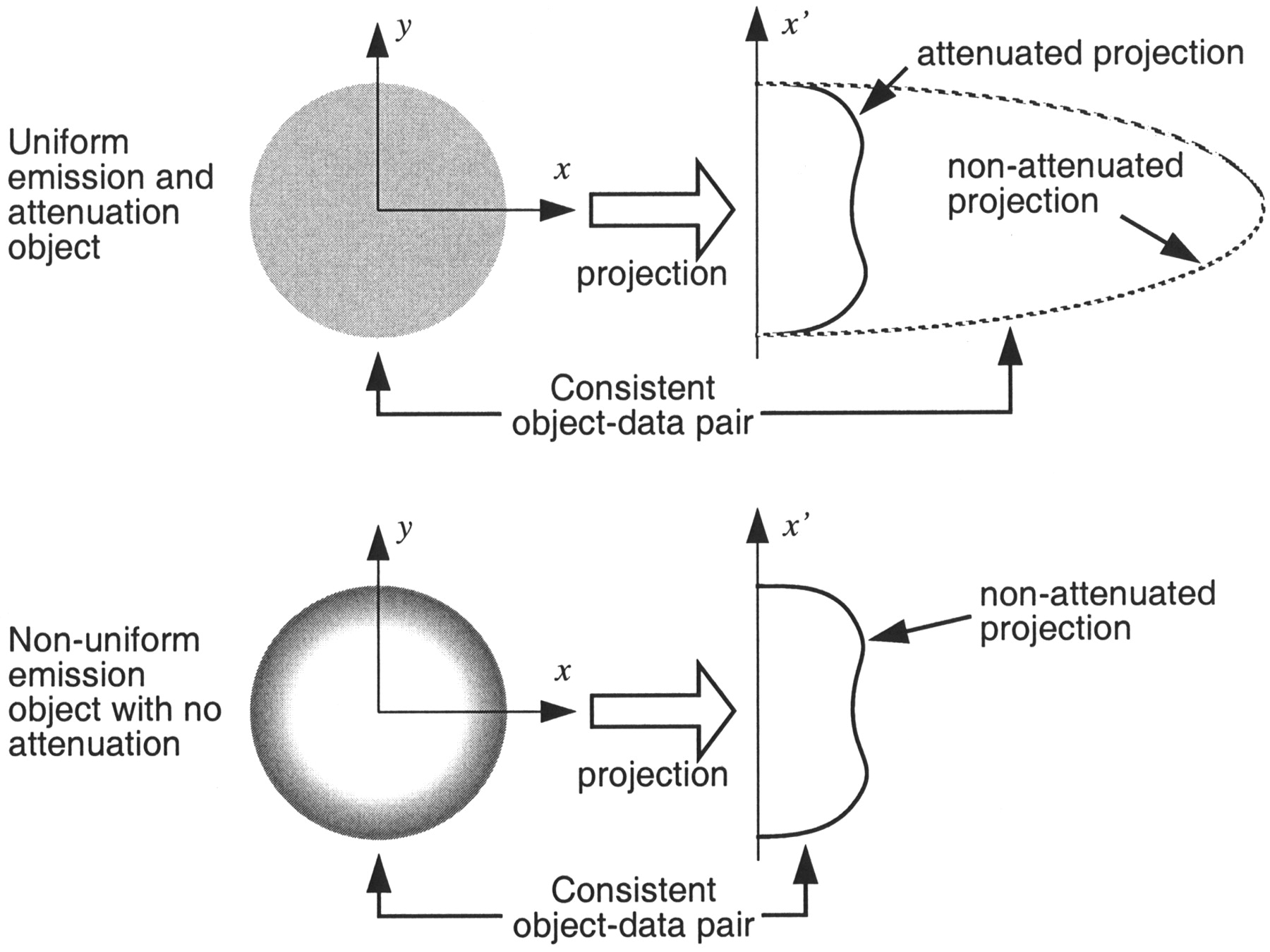
Illustration of how reconstruction without attenuation correction for uniform objects gives rise to images with reduced or even negative tracer concentrations. Nonuniform object is consistent with projections if attenuation is not accounted for.
Because, in general, s(x,y) < 0, the local background around a tumor is reduced, or even negative, which increases the local contrast of tracer foci. With uniform attenuation, it is possible to evaluate Equation 1 directly. This is demonstrated in Figure 2 for an ellipse with dimensions approximating a human abdominal cross-section and with a uniform linear attenuation coefficient of 0.096/cm. The ellipse has a uniform background emission activity of 1.0 arbitrary units (a.u., similar to standardized uptake value [SUV]) and 3 embedded hot spots of 4.0 a.u.
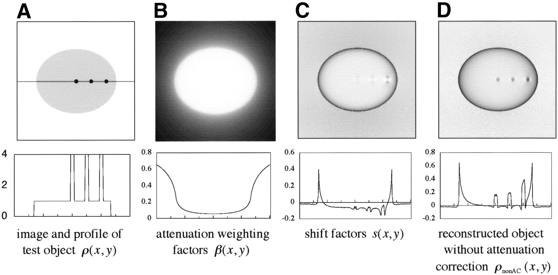
Appearance of images reconstructed without attenuation correction for uniformly attenuating objects, such as abdomen. Top row shows images corresponding to terms in Equation 1, including ρ(x,y) (A), β(x,y) (B), s(x,y) (C), and ρnonAC(x,y) (D). Bottom row shows profiles along the line in top image A.
In the ideal case of noiseless data and continuous sampling, reconstruction of the attenuation-corrected sinogram will reproduce the emission image ρ(x,y) in Figure 2A. The image reconstructed without attenuation correction, ρnonAC(x,y) in Figure 2D, is quantitatively inaccurate in a complex spatially varying manner because of the AW factors β(x,y) and the shift factors s(x,y). The local background for the central hot spots, however, is essentially zero (or even negative), thus making the contrast of the hot spot infinite (if negative image values are truncated, otherwise the contrast is undefined). This illustrates that in regions of uniform attenuation, such as the abdomen, not performing attenuation correction can improve local contrast. The amount of contrast improvement, however, varies in a spatially varying manner, and it would be difficult to accurately predict ρ(x,y) from ρnonAC(x,y), that is, estimating the true distribution from the image without attenuation correction. In addition, the improvements in local contrast can be lost if the entire range of tracer concentration is displayed, as illustrated in Figure 2D. Finally, the apparent benefits in contrast must be balanced against the change in noise levels. Nuyts et al. have demonstrated that not including attenuation correction can decrease the signal-to-noise ratio (SNR) for FBP (27).
Theory of Nonuniform Attenuation
With nonuniform attenuation, it is more difficult to evaluate Equation 1 in a straightforward manner to predict the appearance of images reconstructed without attenuation correction. We can, however, demonstrate a zero-contrast artifact with a noiseless 2D simulation of a human-sized thoracic test object with linear attenuation coefficients μ(x,y) (Fig. 3A) and relative tracer densities ρ(x,y) (Fig. 3B). For illustration, the simulation included regions corresponding to soft tissue (μ = 0.096 cm−1, ρ = 1 a.u.), lungs (μ = 0.048 cm−1, ρ = 0.5 a.u.), spine (μ = 0.192 cm−1, ρ = 0), and myocardium (μ = 0.096 cm−1, ρ = 3.5 a.u.). Reconstruction with 2D FBP of the sinogram without attenuation correction produces the image shown in Figure 3C, which illustrates the well-known artifacts of elevated tracer concentration in the lungs and skin.
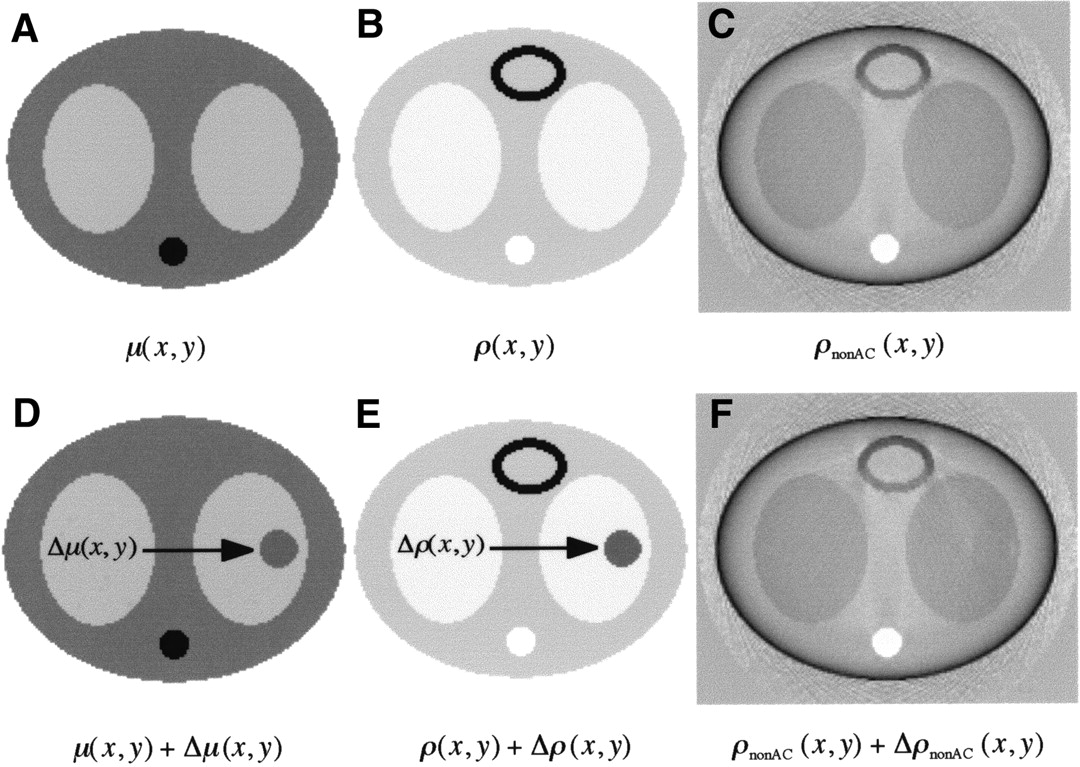
Effect on reconstructed image of not performing attenuation correction for object with nonuniform attenuation, such as thorax. Shown are original object, with attenuation μ(x,y) (A) and emission ρ(x,y) (B), which result in image ρnonAC(x,y) (C) if attenuation correction is not applied. Also shown are the original-attenuation object with added object of equivalent soft-tissue density, Δμ(x,y) (D) and corresponding change in tracer distribution, Δρ(x,y), from Equation 2 (E). The resulting image reconstructed without attenuation correction, ρnonAC(x,y) + ΔρnonAC(x,y) (F), is indistinguishable from image ρnonAC(x,y) (C).
In Figure 3D, a small mass Δμ(x,y) of constant soft-tissue–equivalent density (μ = 0.096 cm−1) is added to the right lung as shown. We assume the change in tissue density is confined to a bounded region Ω, although the value of Δμ(x,y) does not need to be constant within Ω. We can calculate the effect of this perturbation on the attenuated sinogram with the line-integral projection operator P{ }, defined by sf(xr, θ) = P{f(x,y)} =
 , where (xr, yr) are the (x,y) coordinates rotated counterclockwise by an angle θ, and sf(xr, θ) is the sinogram projected from f(x,y).
In 2D imaging, P{ } is equivalent to the radon transform. With this notation we can describe the attenuated sinogram, sμρ(xr, θ), as:

The effect of the attenuation perturbation Δμ(x,y) can then be described by:

We then determine what change to the emission object Δρ(x,y) will, when combined with the modified attenuation object μ(x,y) + Δμ(x,y), yield the same attenuated emission sinogram as in the original case, that is, sμρ(xr, θ) = s(μ+Δμ)(ρ+Δρ)(xr, θ). This leads to the condition:

In other words, for sμρ(xr, θ) to remain unchanged as the attenuation perturbation Δμ(x,y) increases, the change in the emission object Δρ(x,y) must also increase to compensate. To quantify the critical amount of change Δρ(x,y), we simplify this to:
 Eq. 2
Eq. 2
The sinogram P{Δρ(x,y)} does not, in general, satisfy the consistency conditions for the 2D radon transform (28), and therefore this sinogram does not necessarily correspond to any real object Δρ(x,y). The inconsistent part of this sinogram is small, however, for a typical Δμ(x,y), and we can reconstruct the sinogram to estimate a Δρ(x,y) that almost exactly satisfies Equation 2.
A more realistic condition is that in which the changes to both the tissue density Δμ(x,y) and the emission distribution Δρ(x,y) are confined to the same bounded region Ω, such as might be the case for a solitary pulmonary nodule.
For the density change Δμ(x,y) (Fig. 3D), the corresponding Δρ(x,y) from Equation 2 truncated to the region Ω is shown in Figure 3E, superimposed on ρ(x,y). The mean value of Δρ(x,y) within the support of Δμ(x,y) is approximately 2.0 a.u., although this value will depend on Δμ(x,y). Reconstruction of the modified sinogram s(μ+Δμ)(ρ+Δρ)(xr, θ) without attenuation correction produces the image shown in Figure 3F, which has only subtle differences from Figure 2C. The maximum difference between Figures 3C and 3F is approximately 9% of the maximum value. In other words, from reconstructions without attenuation correction, it is not possible to distinguish between the true tracer distributions ρ(x,y) (Fig. 3B) and ρ(x,y) + Δρ(x,y) (Fig. 3E).
A surprising but important aspect of the Δρ(x,y) image is that the nonzero values are roughly localized to the same region Ω as the original change in tissue density Δμ(x,y). This can be understood by noting in Equation 2 that since Δμ(x,y) = 0 outside the bounded region Ω, then P{Δμ(x,y)} = 0, and therefore also the sinogram in the right-hand side of Equation 2 will be zero for all lines not crossing Ω. If consistent, such a sinogram would correspond to an object Δρ(x,y) that vanishes outside Ω. The residual values outside Ω visible in Figure 3E are due to the fact that the sinogram P{Δρ(x,y)} is not perfectly consistent. If we constrain the change in emission distribution to exactly the same region as the change in tissue density, such as might be the case for a solid lung tumor with elevated uptake of 18F-FDG, there are residual differences in the image without attenuation correction, as can be inferred from Figure 3E. With only modest levels of statistical noise, however, these residual differences are not visible, as is shown in the experiment below and can be demonstrated with simple simulations (24). In summary, for regions of nonuniform attenuation it is impossible to predict the true tracer distribution ρ(x,y) from the image reconstructed without attenuation correction, ρnonAC(x,y).
MATERIALS AND METHODS
To verify the predictions of Equation 2, we performed a phantom experiment and analyzed a suitable patient study.
Phantom Study
We used an anthropomorphic torso phantom (Data Spectrum). The liver chamber was filled with water without any activity. The main cavity of the torso was filled with 1.67 kBq/mL 18F-FDG (109-min half-life). The lung chambers contained Styrofoam (The Dow Chemical Co.) beads with a filling fraction of 40%, resulting in an activity concentration of 0.67 kBq/mL. Spheres with inner diameters of 3.4 cm (20-mL net volume) and 1.8 cm (2-mL net volume) were put into the left and right lung chambers to simulate solid lung tumors. The spheres were filled with 34.41 kBq/mL 11C in solution (20-min half-life).
The phantom was scanned in an ECAT HR+ PET scanner (Siemens/CTI) (29), starting 50 min after the phantom was filled. Data were acquired dynamically with fifty 2-min time frames. A 30-min transmission scan was acquired 4 h after the emission scan. All data were acquired in 2D mode. For each time frame, emission images were reconstructed using 2D FBP with and without attenuation correction. Image frames were summed in groups of 3 consecutive 2-min time frames to obtain dynamic images of 6 min per frame.
Patient Study
A female patient was injected with 259 MBq of 18F-FDG. After a 60-min uptake period, the patient was scanned using an ECAT ART scanner (Siemens/CTI) (30). A 10-min emission scan and a 3-min single-photon postinjection transmission scan were collected for each bed position. The ECAT ART scanner collects only emission data in 3D mode, whereas the transmission scan used a slice-collimated single-photon source (7). The transmission image was reconstructed with FBP, whereas the emission images were reconstructed using Fourier rebinning (FORE)+AWOSEM with attenuation correction and FORE+OSEM without attenuation correction (17).
RESULTS
Phantom Study
The images over the critical contrast period are shown in Figure 4, where the large sphere is clearly visible in the images with attenuation correction and in the earliest (highest contrast) frame of the images without attenuation correction. With increasing time, however, the sphere is no longer visible in the images without attenuation correction because of the reduction in contrast due to the faster decay of the 11C relative to the 18F. The large sphere was visible at all contrast levels in the images with attenuation correction. The small sphere was marginally visible in several of the attenuation-corrected images, but without attenuation correction it was visible only in the highest-contrast image.

Dual-isotope phantom experiment with 11C in spheres (arrows) in lungs and 18F in lungs and thorax. From left to right, images are sequential 6-min time frames. Top row is with attenuation correction; bottom row is without attenuation correction.
Patient Study
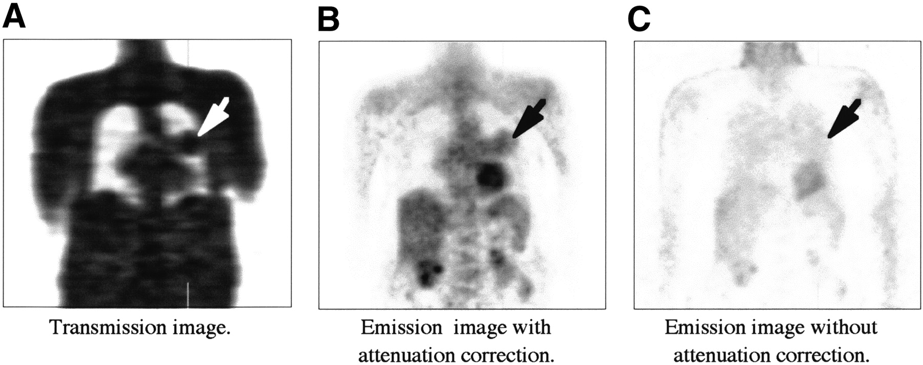
Figure 5 shows coronal sections of the reconstructed images of the patient study. A mass with a volume of approximately 65 cm3 in the left lung of the patient was present in transmission images. A hamartoma seen clearly in the attenuation-corrected images is not seen in the images without attenuation correction. The average SUV of the tumor was 2.1. The emission images were also reconstructed with FBP, but other than an apparent increase in statistical noise, there was no significant change in the images.

Coronal sections of whole-body images of patient with hamartoma (arrow), which is clearly visible as dense object in transmission image (A) and shows uptake of 18F-FDG in attenuation-corrected emission image (B). In same image plane of emission image reconstructed without attenuation correction (C), however, hamartoma is not detectable.
DISCUSSION
The attenuation effect in PET is nonlinear. Images reconstructed without attenuation correction can give misleading impressions of the true tracer distribution, particularly for the general situation of nonuniform attenuation that occurs in whole-body PET oncology imaging. In the thorax, for example, it is widely observed that image reconstruction without attenuation correction results in the appearance of lungs with higher uptake than muscle and even in the appearance of negative tracer concentrations in mediastinal regions. With attenuation correction, however, the relative uptake of tracers in the lungs and in the nearby soft tissue is correctly recovered (31).
Several studies have attempted to heuristically determine the effect of not performing attenuation correction on detection (1–3,32), localization, or shape distortion (33) and even quantitation (34,35). In the simpler case for PET, we can use Equation 1, which was independently derived by Nuyts et al. (27,36), to analytically describe the appearance of images reconstructed without attenuation correction (for FBP). With Equation 1, we demonstrated that for regions of uniform attenuation, such as the abdomen, images without attenuation correction have locally enhanced contrast, because of a background subtraction effect (25). A caveat is that the amount of contrast enhancement in uniformly attenuating regions varies with position in a complicated manner.
The results for images reconstructed with FBP presented here, which allow negative values, do not apply to images reconstructed by iterative methods, such as OSEM (37), which have nonnegativity constraints. Thus, images without attenuation correction reconstructed by FBP or OSEM can have very different appearances. If iterative image reconstruction is desired, say, for suppression of streak artifacts, an iterative algorithm that correctly treats negative values, such as the maximum-likelihood algorithm allowing negative reconstruction values (NEG-ML) developed by Nuyts et al. (27,36), should be used instead of OSEM.
In regions of nonuniform attenuation, such as the thorax, the effects of not performing attenuation correction are more complex and difficult to generalize from Equation 1. It is possible to show, however, that a tumor can “disappear” in images reconstructed without attenuation correction. This occurs when the increased attenuation caused by a solid tumor in the lungs is precisely compensated by increased tracer uptake. In this case, the sinogram without attenuation correction is identical to one in which the lung mass is not present. Thus, reconstruction of the sinograms will yield identical images, as illustrated by Figures 3C and 3F. The critical standardized uptake value for the zero-contrast effect depends on the size, location, and density of the tumor. This effect is independent of the noise level and the image reconstruction method, as Equation 2 indicates that the tumor-present zero-contrast effect is due to having a sinogram identical to that in the tumor-absent case.
CONCLUSION
The results indicate that all whole-body studies should be reconstructed with attenuation correction to avoid missing regions of elevated tracer uptake in the lungs.
APPENDIX
We give here the explicit expression of the shift image s(x,y) in Equation 1 and also show that in regions of uniform attenuation, such as the abdomen, s(x,y) < 0 near the center. We parameterize measured lines of response by the usual sinogram variables xr and θ, where xr is the distance between the line and the origin of the coordinate system (x = y = 0) and the angle θ determines the unit vector along the line as (−sin θ, cos θ). The attenuation coefficient for line (xr, θ) is denoted α(xr, θ) ≤ 1, and the average attenuation at point (x,y) is then simply:
 Eq. 1A
The FBP reconstruction of the attenuated radon transform a(xr, θ) · ρ(xr, θ), without attenuation correction, is:
 Eq. 2A where h(xr) denotes the ramp filter kernel (the inverse Fourier transform of the apodized ramp filter), and p(xr, θ) the nonattenuated radon transform of ρ(x,y).
By replacing p(x cos θ + y sin θ − xr, θ) in Equation 2A by its expression as a (nonattenuated) line integral of ρ(x,y), and by using the linearity in p and hence in ρ, we see that ρnonAC can be rewritten in the form:
 Eq. 3A and by defining s(x,y) =
 R2 k(x, y, x′, y′)ρ(x′, y′)dx′dy′, we have Equation 1.
To find the expression for the spatially varying convolution kernel k, we use again the linearity of Equation 2A by applying it to a unit point source located at (x0, y0), that is, ρ(x,y) =δ(x − x0)δ(y − y0). The corresponding sinogram is p(xr, θ) = δ(x0 cos θ + y0 sin θ − xr), which when substituted in Equation 2A yields:
 Eq. 4A
If a point (x,y) is located in the center of a uniformly attenuating object, then any other point (x′, y′) has lower attenuation, and therefore in Equation 4A one has a(x′ cos θ + y′ sin θ, θ) ≥ β(x,y). Since h(xr) < 0 for xr < 0, we conclude that for the central point (x,y) the kernel is negative, that is, k(x, y, x′, y′) < 0 and therefore s(x,y) < 0 at or near the center of a uniformly attenuating object as illustrated by Figure 1C.
Acknowledgments
We appreciate discussions of this work with Drs. Richard L. Wahl, Johan Nuyts, Hubert Vesselle, and Rolf Clackdoyle. This work was supported by grant CA-74135 from the National Institutes of Health.
Footnotes
Received Dec. 26, 2001; revision accepted Jul. 3, 2003.
For correspondence or reprints contact: Paul E. Kinahan, PhD, University of Washington Medical Center, Box 356004, 1959 NE Pacific St., Seattle, WA 98195-6004.
E-mail: kinahan{at}u.washington.edu


