


Abstract
Quantitative gated SPECT (QGS) software has been reported to overestimate the left ventricular ejection fraction (LVEF) in patients with small hearts. This finding is caused by the inaccurate detection of the endocardial surface of the left ventricle (LV) due to low resolution and partial-volume effects. In this article we develop a method to calculate the LVEF from gated SPECT data without edge detection and compare it with the QGS method of calculating the LVEF. Methods: The short-axis images were transformed to the prolate spheroid coordinate system, and detection of the layer of maximum counts (a surface area of maximum counts) was made. First, the volume enclosed by the layer of maximum counts (Vmax) was calculated; then the corresponding ejection fraction [(LVEF)max] was calculated. The LVEF was calculated by multiplying the (LVEF)max by a constant factor, which was determined from a series of calculations made using QGS on larger hearts. In computer simulations the end-diastolic left ventricular volume (EDV) and the targeted LVEF (tLVEF) were varied to produce LVs of different sizes. The LVs were modeled by 2 confocal hemiellipsoids with 7 different EDVs. The tLVEF was increased from 25% to 75%, in 5% step-size increments, for a total of 11 different ejection fractions. These datasets were then smoothed, creating a total of 77 smoothed sets. The smoothed images were processed by the QGS method and by our method. In patient studies, 58 patient datasets were processed by the QGS method and by our method. No attenuation correction was performed on these datasets. The patients were divided into 2 groups: 44 patients with large hearts (EDV ≥ 80 mL) and 14 patients with small hearts (EDV < 80 mL). Results: In computer simulations, the QGS method and our method performed well when imaging large EDVs (EDV ≥ 80 mL). Our method derived better results than did the QGS method for small EDVs. In patient studies the LVEF calculated by our method matched well with the QGS LVEF in the 44 patients with large hearts. The correlation coefficient between them was found to be 0.957. Of the 14 patients with small hearts, the LVEFs of 5 patients were severely overestimated by the QGS method compared with the results obtained with our method. Conclusion: It is possible to calculate the LVEF without edge detection. Compared with QGS LVEF, our method gave better results for small LVs in computer simulations.
Gated SPECT (gSPECT) offers the possibility of simultaneous measurement of heart perfusion and myocardial function. Values of the left ventricular ejection fraction (LVEF), heart wall thickening, and heart wall motion are important factors in the diagnosis of coronary artery disease and the prognosis of patient recovery. Also, the determination of the LVEF using nuclear ventriculography is an important tool for diagnosing dysfunction of the left ventricle (LV), which is related to several diseases of the myocardium. A particular problem in using gSPECT is the low spatial resolution that results in overestimation of the LVEF in small hearts. Most methods implemented on commercial SPECT systems use edge-detection schemes in the calculation of the LVEF. However, edge-detection schemes are especially susceptible to partial-volume effects, which become more severe when imaging small hearts. The calculation of the LVEF in small hearts can be improved using methods, such as the one proposed in this article, that are less sensitive to partial-volume effects and enable calculation of the volume (Vmax) enclosed by the layer of maximum counts (a surface of maximum counts).
gSPECT using 99mTc-labeled pharmaceuticals (1–4) and 201Tl (4,5) has been used to estimate functional parameters for quite some time. However, because of the very low resolution of gSPECT, which is comparable to the thickness of the heart wall, accurate measurement of parameters such as the ejection fraction is not possible. To calculate functional parameters such as the LVEF, heart wall thickening, and heart wall motion from gSPECT, edges of the heart are determined using the current commercial quantitative gSPECT software package ([QGS]; Cedars-Sinai Medical Center, Los Angeles, CA) (6,7). Then, on the basis of the position of the edges, all functional parameters are determined. Because of the low spatial resolution of approximately 15 mm, the endocardial edges at the opposite sides of the LV cavity overlap. As a result the position of the calculated edge appears to be closer to the center of the cavity. (The temporal resolution has less of an effect because most gSPECT studies are digitized into 16 time frames of approximately 0.05 s, depending on the heart rate.) This is particularly a problem for end-systolic configuration because the volume of the LV is at its smallest and the endocardial edges are at their closest points. This is most problematic in low-resolution images and images of patients with small hearts. Incorrect determination of the position of the edges results in underestimation of the end-systolic volume (ESV), which results in overestimation of the LVEF (8–10). In this article, this effect is referred to as small heart error.
Instead of calculating endocardial edges, we propose a method for calculation of the LVEF based on the calculation of the layer of maximum counts. The layer of maximum counts is defined as follows: If one determines the maximum counts along each radius in the short-axis slices, a circumferential curve that inscribes an area that includes a cross section of the intraventricular blood pool and an internal portion of the LV wall is derived. If we do this for each short-axis slice from its apex to its base, a circumferential surface is defined. This surface is referred to as the layer of maximum counts.
In this article, a technique that involves determining the position of the layer of maximum counts surface and using it to calculate the LVEF is developed and implemented. The technique does not require detection of edges for the calculation of functional parameters such as the LVEF. The technique suffers less from resolution effects because in short-axis slices there is a greater distance between the opposing walls of the layer of maximum counts of the LV than there is between the opposing walls of the endocardial surface. The layer of maximum counts is usually closer to the midventricular surface than to the endocardial surface.
MATERIALS AND METHODS
Calculation of Vmax
To calculate the Vmax, the short-axis image of LV was transformed into the prolate spheroid coordinate system (Fig. 1) (11). In the prolate spheroid coordinate system the horizontal ξ-axis direction lies along the transmural direction, so it goes “through” the LV wall. The φ-axis (φ-axis, Fig. 1) is the circumferential angle that ranges from 0 to 2π and the θ-axis is the azimuthal angle that ranges from 0 to π. In each short-axis image the location of the maximum counts ξmax(θ,φ) was searched for along the ξ-axis for fixed coordinates θ and φ in the prolate spheroid coordinate system. Because the heart is not entirely ellipsoid, but rather is truncated at some θmax, θmax is dependent on the value of φ. The value θmax(φ) was found by thresholding the image at 50% (11).
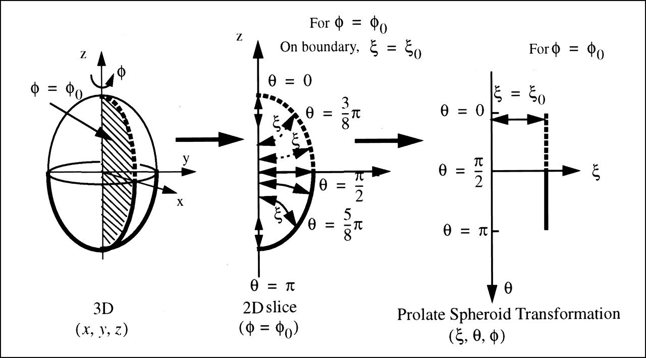
Prolate spheroid transformation of ellipsoid. (Left) A 3D ellipsoid in Cartesian coordinate system. (Center) Half of 2D vertical slice through ellipsoid. (Right) Prolate spheroid transformation of 2D slice in Center.
The Vmax is calculated by:
 Eq. 1
Eq. 1 where J is the Jacobian of the prolate spheroid transformation. The focal length C is a parameter related to the prolate spheroid transformation. It was found that the calculated volume Vmax is not sensitive to the value of C within the range of physiologic heart sizes (11).
Estimation of LV Cavity Volume and LVEF
Assuming that the layer of maximum counts is located at a fixed position within the wall of the LV myocardium, due to certain smoothing processes, the LV cavity volume Vc is estimated by calculating the Vmax and then subtracting the volume of the myocardium enclosed by the layer of maximum counts. The part of the LV myocardium that is enclosed by the layer of maximum counts has a volume of Vmyo−en, whereas the entire volume of the LV myocardium is denoted as Vmyo. The ratio α = Vmyo−en/ Vmyo is assumed to be constant for each particular image smoothing process. It follows that:
 Eq. 2 where β = Vmyo/ Vc.
The LVEF is defined by:
 Eq. 3 where the subindices ED and ES stand for quantities measured at end diastole and end systole. Using Equation 2 we can rewrite Equation 3 as:
 Eq. 4 or
 Eq. 5
Eq. 5
The myocardium is assumed to be incompressible because the tissue is incompressible and the tissue volume changes caused by changes in blood volume within the myocardium are negligible factors. This means that it is assumed that the volume of the LV enclosed by the layer of maximum counts is equal for all time gates between end systole and end diastole, and in particular (Vmyo−en)ED = (Vmyo−en)ES, so that the difference of these 2 terms in Equation 5 is 0. Using this fact, Equation 5 can be rewritten as:
 Eq. 6
Eq. 6
Equation 2 is used to obtain the expression [1 + αβ ED], where βED = (Vmyo)ED/ (Vc)ED and α is assumed to be constant throughout the cardiac cycle. The (LVEF)max is calculated directly from the volumes enclosed by the layer of maximum counts:
 Eq. 7
Eq. 7
Our approach to calculating the LVEF is as follows: First the (LVEF)max is calculated and then modified by the factor 1 + αβED (Eq. 6). Coefficients α and βED are known factors in the computer simulations. However, in patient studies they had to be determined. As pointed out earlier, α depends on the imaging method (data acquisition, reconstruction, smoothing, and so forth). For gSPECT images reconstructed with the same software, the reconstructed images were filtered and smoothed by similar processes, so it is reasonable to assume that α remains constant for all patients imaged with the same device. The coefficient β ED stands for the volume ratio of the LV myocardium and the LV cavity at end diastole, which is in a narrow physiologic range. Plotting the LVEF found by another source (such as QGS with large hearts) versus the (LVEF)max, the slope can be found, which should be the value of 1 + αβED for a given imaging system. This same slope should also apply for small hearts as well.
Computer Simulations
Four sets of digital phantoms with different ratios of Vmyo/Vc = β were used to verify Equation 2 and determine the value of α. All of the phantoms consisted of 2 confocal hemiellipsoids with uniform LV myocardial counts. Each set had a fixed β, whereas the targeted cavity volume was increased from 30 to 150 mL, at 15-mL step-size increments. The pixel size was 0.532 cm, which is the common pixel size used in the PRISM 3000XP SPECT system (Marconi Medical Systems, Cleveland, OH). Each phantom was smoothed by applying the 3-dimensional (3D) analog of the familiar “S9” 2-dimensional (2D) low-pass filter (27 total voxels for the real space kernel):
 Eq. 8 For this particular filter the cutoff frequency (the point at which the filter is at one half the maximum power) is 0.195 cycle/pixel, or 0.3665 cycle/cm. Vmax was then calculated and plotted versus the targeted Vc.
Ford et al. (10) developed a series of mathematic LVs by varying the end diastole, the LV end-diastolic volume (EDV), and the targeted LVEF. We developed similar phantoms to evaluate our method of calculating the LVEF and compared our results with the QGS results. As before, the LV was modeled as 2 confocal hemiellipsoids with uniform myocardial counts. A constant ratio was maintained between the axes of the inner hemiellipsoid during the cardiac cycle. The volume of the myocardium was kept constant during the cardiac cycle. The EDV was set to equal the volume of the myocardium (βED = 1, which corresponded to one of the heart sizes of the Mathematical CArdiac Torso phantoms). The targeted LVEF (tLVEF) was chosen such that it would change from 25% to 75% in 5% increments to derive a total of 11 tLVEFs. For each tLVEF, 8 frames of the cardiac cycle were generated using the formula (10) Vi = EDV[tLVEF (cos(iπ/4) − 1)/2 + 1], where i ranged from 0 to 7. The 3D kernel in Equation 8 was then used to smooth these datasets. There were 7 sets of targeted EDVs (before smoothing): 20, 40, 60, 80, 100, 140, and 180 mL Therefore, the total number of datasets was 77. Each dataset was 64 × 64 × 25 × 8.
The LVEF was calculated using our method and using the QGS method on the Marconi Odyssey V4.0D/3.2 computer (Marconi Medical Systems). In calculations of the LVEFs using our method, α and β ED were known from the digital phantom used in the simulation: α = 0.427 and βED = 1.0, so the LVEF = 1.427(LVEF)max. An appropriate Marconi header was added to these datasets before QGS was used to determine the LVEFs for these datasets.
Patient Studies
Fifty-eight sets of gSPECT cardiac patient data were used to study the LVEFs obtained by QGS and by our new method. The patient population included 29 male and 29 female subjects. Most of the patients were referred for the gSPECT study for evaluation of potential ischemic cardiac disease. The findings for most of the patients showed that there was no evidence of ischemia. There were 6 cases with abnormal results: 1 with apical ischemia with associated dyskinesia, 1 with 2 large areas of ischemia involving the mid-to-distal anterior wall and the lateral wall, 1 with a moderate-sized infarct of the posterolateral wall, 1 with an inferior wall infarction with minimal periinfarct ischemia in the proximal inferior wall, 1 with a mildly dilated LV with mild diffuse hypokinesia, and 1 with a dilated LV showing apical ischemia with global hypokinesia.
The cardiac gSPECT data were acquired as follows: Each patient was injected with approximately 888 MBq 99mTc-methoxyisobutylisonitrile. For 23 patients, stress was induced on a treadmill using the standard Bruce protocol. For the other 35 patients, stress was induced pharmacologically. Of these, 13 were stressed using adenosine, 9 were stressed using dipyridamole, 12 were stressed using dobutamine, and 1 was stressed using atropine. One hundred twenty projections over 360° were acquired using a 3-head PRISM 3000XP SPECT system (Marconi Medical Systems) with low-energy, high-resolution, parallel collimators. For each projection angle, the data were acquired and digitized into sixteen 64 × 64 frames over the cardiac cycle. The acquisition was zoomed so that the pixel size was 0.532 cm.
The gSPECT data were reconstructed using the filtered backprojection algorithm with a 1-dimensional ramp filter. A 3D low-pass filter (Butterworth filter: order, 5; cutoff frequency, 0.17–0.21 cycle/pixel) was applied after the projections were reconstructed. No attenuation corrections were made when reconstructing these datasets.
The QGS program was then used to process the reconstructed data. Also, to enable use of our method, the maximum LVEF [(LVEF)max] was calculated. The threshold used in our calculations to determine the θmax (φ) needed for the volume calculations in Equation 1 was one half of the maximum myocardial counts. By cutting out the short-axis LV within a 13-pixel-radius cylinder, we eliminated the potential high counts that may have occurred outside the LV. The focal length C used in the prolate spheroid transformation was 6 pixels for all patient studies.
The patients were divided into 2 groups. The first group consisted of 44 patients with normal or large-sized hearts (EDV ≥ 80 mL). On the basis of this group, the value of 1 + αβED was calculated by linear regression. The second group consisted of 14 patients with small hearts (EDV < 80 mL).
RESULTS
Computer Simulations
In the simulation performed to verify Equation 2, Vmax was calculated and plotted versus the targeted Vc for 4 sets of phantoms with different ratios of Vmyo/ Vc = β (Fig. 2). Each set was fitted to a line through the origin (y = kx). The correlation coefficient was >0.99 for each set. From the slope of the fitted line, the value of α was calculated by α = (slope − 1)/β. For β = 0.8, 1.0, 1.5, and 3.0, the calculated values of α were 0.443, 0.427, 0.429, and 0.401, respectively. The error for α was <10%.

Plot of calculated volume Vmax, volume enclosed by layer of maximum counts, vs. targeted LV cavity volume Vc for 4 sets of phantoms with different ratios between volumes of LV myocardium and volumes of LV cavity (Vmyo/Vc = β).
These results verify that the relationship between Vmax and Vc is indeed a straight line that passes through zero as predicted by Equation 2. Also, if we assume that the slope of the line is related to [1 + αβED], the results show that α (Vmyo−en/ Vmyo) remains fairly constant for different heart sizes and shapes (i.e., different values of β). This result is crucial to the derivation of the result given in Equation 6, which indicates that the layer of maximum counts occurs at almost a fixed depth in the myocardium during the cardiac cycle. The constant value of α makes it possible to estimate the LVEF from Vmax in Equation 2 and the (LVEF)max in Equation 7 even though the value of β changes during a cardiac cycle.
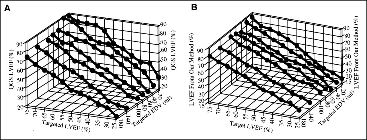
In the simulations performed to calculate the LVEF, 77 smoothed datasets were processed by the QGS method and by our method. For large phantoms (EDV ≥ 80 mL), the QGS LVEF and the LVEF calculated by our method closely approximated the tLVEF. Errors in the QGS LVEF increased as the cardiac volume decreased (EDV ≤ 80 mL) (Fig. 3A; Fig. 4A). Conversely, the LVEF obtained with our method was closer to the tLVEF than the QGS LVEF was in the studies of small hearts (Fig. 3B; Fig. 4B).

Plots of QGS LVEF (A) and LVEF by our method (B) vs. targeted LVEF (tLVEF) and targeted end-diastolic volume (EDV). For phantoms with large EDVs (EDV ≥ 80 mL), QGS LVEF and LVEF by our method closely approximate tLVEF. However, for small hearts (EDV < 80 mL), our method produced better results than did QGS method.

(A) Plot of (difference between QGS LVEF and targeted LVEF [tLVEF]) vs. tLVEF. (B) Plot of (difference between LVEF calculated by our method and tLVEF) vs. tLVEF.
To determine how well the calculated LVEFs matched the tLVEF for each EDV, we calculated the slope of the linear least-squares fit to the plot of the calculated LVEFs versus the tLVEFs. A linear least-squares fit was performed for each dataset in Figures 3A and 3B using XMGR (copyright 1996–1998; ACE/gr Development Team; http://plasma-gate.weizmann.ac.il/Xmgr/). To achieve perfect agreement between the calculated LVEFs and the tLVEFs, the slope of the fitted line should be unity. If there is a large discrepancy between the fitted slope and unity, the calculated LVEFs will lack agreement with the tLVEFs. For EDVs = 20, 40, 60, 80, 100, 140, and 180 mL, the slopes for the QGS results were 1.289, 1.255, 1.166, 1.055, 1.018, 0.9823, and 0.9528, whereas the slopes for our results were 1.085, 1.096, 1.040, 1.078, 1.062, 1.023, and 1.046. Our method gives better results when imaging small hearts (EDV < 80 mL).
Patient Studies
Values of the LVEFs from 58 patients were calculated using the QGS method and our method. Figure 5 shows the QGS LVEFs of the 44 patients with large hearts versus the (LVEF)max calculated by our method. The linear coefficient 1 + αβED of the least-squares fit was 1.226. Using Equation 6, we arrived at αβED = 0.226. We calculated the difference between the LVEFs obtained using our method and the QGS LVEFs and plotted the histogram in Figure 6.

For 44 patients with large EDVs (EDV ≥ 80 mL), plots of QGS LVEF vs. (LVEF)max by our method. Slope of fitted line is used to calculate LVEF.
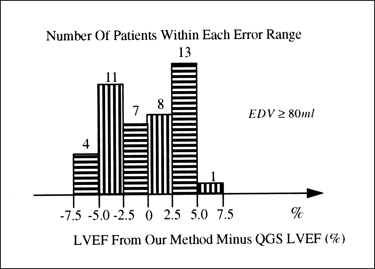
Histogram shows difference between LVEFs obtained with our method and those obtained with QGS LVEF method for 44 patients with large hearts (EDV ≥ 80 mL).
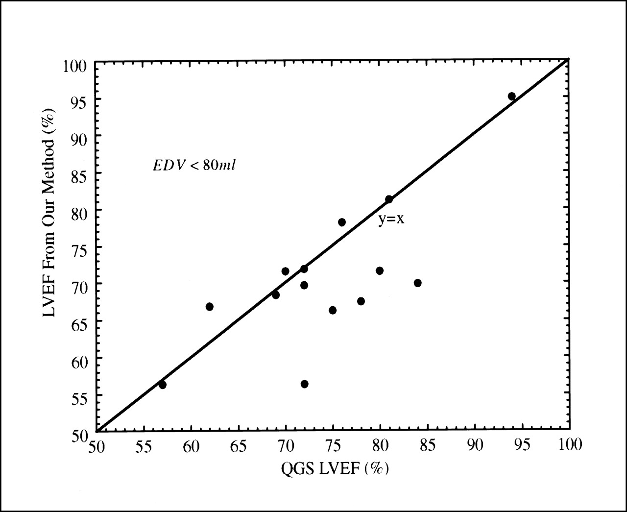
For the 14 patients with small hearts (EDV < 80 mL), the LVEFs obtained using our method were plotted versus the QGS LVEFs in Figure 7. There were 5 patient studies in which the LVEFs calculated by QGS were determined to be overestimated by >9% compared with the LVEFs obtained using our method. The EDVs for these patients were 62, 52, 69, 59, and 49 mL. For the patients with small hearts, the average heart size [(Vc)ED] was 64 ± 11 mL. Therefore, these 5 patients were not necessarily the ones with the smallest hearts, but their hearts did tend to be of the smaller sizes and had ejection fractions of >70%. Larger hearts with higher ejection fractions tended to fit closer to the fitted regression line.

For 14 patients with small EDVs (EDV < 80 mL), plots show LVEFs by our method vs. QGS LVEFs. Five patients had severely overestimated LVEFs (>9%) obtained by QGS LVEF method compared with LVEFs obtained by our method.
DISCUSSION
A method for calculating the LVEF without calculating the edges of the endocardial wall of the LV in gSPECT images was developed. The method improves the accuracy of calculating functional parameters from gSPECT in patients with small hearts. The method requires calculating the regression slope of Vmax versus Vc for large hearts using software such as the QGS software package. The slope of this regression curve was used to develop a formulation for the calculation of the LVEFs of smaller hearts, using the layer of maximum counts. Compared with QGS, our method gave better results for small LVs in computer simulations. In patient studies, QGS overestimated the LVEFs in small hearts by >9% compared with those obtained with our method. This study concentrated on the calculation of the LVEF but the extension of this method to calculating other parameters such as heart wall thickness would not be difficult.
Our method is based on 2 assumptions. The first assumption is that the layer of maximum counts remains at a fixed position in the LV myocardium for 1 imaging system during the heart cycle. Using the computer simulation results presented in this work, the ratio between the volume enclosed by the layer of maximum counts and the volume of the LV myocardium (α) is constant when the same smoothing filter is applied to each phantom. This is true for any heart size (Fig. 2), which means that α can be treated as a constant in any single imaging system in which each patient dataset is processed using the same reconstruction method. The second assumption is that the volumetric ratio between the LV myocardium and the cavity at end diastole is within a narrow physiologic range for all patients. The strong linear agreement and close correlation (r = 0.957) between the LVEF calculated by our method and that calculated by the QGS method (Figs. 5 and 6) proves that this is a good assumption for the subset of patients studied in this investigation.
If the second assumption is invalid, such as in cases of systolic or diastolic dysfunction, our method will still result in relatively small errors. For normal hearts we obtained αβED = 0.226, where βED is the ratio between the myocardium volume and the EDV. For a heart with disease (systolic or diastolic dysfunction), βED may change significantly from normal values, but the calculation of the LVEF using Equation 6 will be affected to a much less extent because α is <1 (0.226 if we assume β ED = 1). For example, for a heart with a systolic dysfunction such as dilated cardiomyopathy (LVEF decreases, LV EDV increases), βED can decrease to half of its normal value because of the increased EDV. In this case the value for 1 + α βED could be 1.113 instead of 1.226. The relative error of the LVEF caused using 1 + αβED = 1.226 is 10%. On the other hand, for a heart with diastolic dysfunction such as hypertrophic cardiomyopathy or restrictive cardiomyopathy (LVEF increases, LV EDV decreases), βED can increase to twice its normal value because of the decrease of the EDV or the increase of the volume of the myocardium. In this case the value for 1 + αβED could be 1.452 instead of 1.226. The relative error of the LVEF caused using 1 + αβ ED = 1.226 is −16%.
In images obtained with gSPECT, the edges of the LV are blurred by the smoothing process when very noisy data are reconstructed, which results in the small heart error described earlier. Contrary to the conventional segmentation method used in the LVEF calculations, our method detects the layer of maximum counts of the LV myocardium, which is less affected by the small heart error. The position of the layer of maximum counts is basically not affected by this error. We found that if the EDV > 80 mL the measurements of the calculated LVEF were not affected by the small heart error. On the other hand, when the positions of the edges were used to determine the ejection fraction (QGS), the accuracy dropped rapidly when small hearts were simulated. This is in agreement with previous work (10).
It is anticipated that in severe perfusion defects it will be easier to calculate the area of the layer of maximum counts than it is to determine edges that are missing, which are needed in standard software for calculating the LVEF. We point out that this is conjecture and still needs to be verified. For normal hearts, the area of the layer of maximum counts is as easy to calculate as the enclosed volume. We have shown in computer simulations that the area correlates perfectly in a linear fashion with the volume (11). With abnormalities in the LV some interpolations must be done to define the LV cavity in standard methods. With area calculations this is not necessary because it is implicitly assumed that the location of the maximum counts in the defect will be the same as those where the tissue is normal. It is expected that this will not be true in all cases, but it is expected to hold true in most cases. However, this needs to be verified for defects of various sizes and at various locations. This might be very important in the case of hearts with large defects where accurate estimation of the LVEF is very difficult to obtain with standard methods. Therefore, when using areas it is expected that the accuracy of the LVEF measurements will be better in cases of severe abnormalities, if not at least as good as volume calculations of normal hearts using conventional software. For the same reason, we expect this method to work better in cases of dyskinesia.
CONCLUSION
We have presented a method to calculate the LVEF without edge detection. Compared with QGS LVEF, our method gave better results for small LVs in computer simulations. In patient studies, our method gave results similar to those of the QGS method when imaging patients with large hearts. On the basis of our computer simulations, one can infer that our method gave more accurate measurements of the LVEF when imaging patients with small hearts, whereas the QGS method overestimated the LVEF.
Acknowledgments
The authors thank Sean Webb for editing the manuscript, Paul Christian for providing the patient data, and Dr. G. Larry Zeng and Kerri Harris for technical assistance. This work was supported by National Institutes of Health grant RO1 HL39792.
Footnotes
Received Sep. 24, 2001; revision accepted Jan 31, 2002.
For correspondence or reprints contact: Bing Feng, MS, Medical Imaging Research Laboratory, Center for Advanced Medical Technologies, University of Utah, 729 Arapeen Dr., Salt Lake City, UT 84108-1218.
E-mail: bfeng{at}doug.med.utah.edu
In this issue


Jump to section
Related Articles
Cited By...
- Left Ventricular Function Assessment Using 2 Different Cadmium-Zinc-Telluride Cameras Compared with a {gamma}-Camera with Cardiofocal Collimators: Dynamic Cardiac Phantom Study and Clinical Validation
- Quantifying Transient Ischemic Dilation Using Gated SPECT
- Calculation of Ejection Fraction in Gated SPECT