


Abstract
A tool was developed for automated intrapatient comparison of brain SPECT images, with specific emphasis on gray-level normalization. Methods: Ictal and interictal 99mTc-ethyl cysteinate dimer SPECT images were acquired for 6 children with partial epilepsy (age range, 2–10 y). For each patient, 3-dimensional rigid geometric ictal-to-interictal image registration optimizing different classic criteria (correlation coefficient, ratio uniformity) in a multiscale translation–rotation 6-parameter space was first performed. Gray-level normalization was then performed with different methods, using a 1- or 2-parameter linear model. In the 1-parameter case, the scaling factor was equal to the interictal-to-ictal ratio of the maximum, mean, or median values calculated within different reference volumes (whole brain or cerebellum) or obtained by linear regression between ictal and interictal counts in the brain or by maximizing a robust criterion, the number of deterministic sign changes in the subtraction images. In the 2-parameter case, the scaling factor and additive constant were estimated using these last 2 methods. For each patient, registration validity and normalization plausibility were assessed by considering the correlation scatterplot together with the different normalization lines and by comparing interictal and registered normalized ictal images using a twin display (with isocontours) in the 3 orthogonal planes. Three-dimensional volumes of interest could be selected on coupled interictal–subtraction images for further focused numeric comparison. Results: After a satisfactory and stable geometric registration with both criteria, the different normalization methods led to similar subtraction images for 5 of 6 patients, except the maxima ratio, which gave noticeably different results in 2 patients. For the remaining patient, with highly dissimilar ictal–interictal images, the maxima ratio normalization was obviously wrong and the other 1-parameter methods probably better depicted the data than did the 2-parameter methods. Conclusion: When comparing intrapatient brain SPECT images, one should be aware of the potential impact of the gray-level normalization method on clinical interpretation. For ictal–interictal images, simple robust scaling should be recommended. In particular, image maximum should generally not be considered a valid reference, and no additive constant is needed in the linear gray-level normalization model.
Intrapatient comparison of brain SPECT images remains an incompletely solved problem. Indeed, whereas many geometric registration methods have been validated (1–5), gray-level normalization remains debated. It has been addressed for various diseases, for both intrapatient and interpatient SPECT and PET comparison, in terms of normalization factor (6), intensity scaling, reference region choice (7–9), and global (region-independent) effect removal (10). For the comparison of only 2 consecutive scans acquired for 1 patient, in which average and variance values cannot be estimated at the pixel level, normalization can be formulated in terms of the reference region problem. This reference region should be understood in a wide sense, as a 3-dimensional (3D) subset of connected or nonconnected stable voxels, ranging from 1 voxel to the whole dataset, which is selected on the basis of physiologic knowledge or statistical properties. The basic assumption is that, from this set of voxels, a global gray-level transformation between the 2 scans can be derived that allows local changes to be exhibited through direct comparison or subtraction. The main purpose of this study was to compare different normalization methods that are commonly or rarely used and characterized by different degrees of robustness. Interictal and ictal images from epileptic patients were used as a test set.
MATERIALS AND METHODS
Patients and Data
Ictal and interictal 99mTc-ethyl cysteinate dimer SPECT images of children with partial epilepsy were used. Six well-documented patients, aged 2–10 y, were selected from a previous study on subtraction ictal SPECT that included 27 children (11). These 6 patients were not selected on a clinical basis. They were chosen to provide a sample of the various types of difference images that were present in the initial series, representative with respect to the spread and amplitude characteristics of the apparent differences. There was variable involvement of the whole brain in 1 patient, at least 1 more or less diffuse focus in 3 patients, and no visible difference in 2 patients. Besides the information from the SPECT images, information about the location of the epileptic focus was variably available from clinical seizure; ictal videoelectroencephalography; MRI; or, in 2 patients, electrocorticography. Patient characteristics are listed in Table 1. Image acquisition details can be found elsewhere (11).
Patient Characteristics
Image Preprocessing
Image Transfer and Conversion.
Ictal and interictal axial slices (128 × 128 × 128 matrix) were sent from Rouen to Reims in the Interfile format (version 3.3). They were then converted to the Park format (Park Meditech Inc., Farnborough, U.K.) and sent to a Sun 4 (Sun Microsystems, Mountain View, CA) computer. Pairs of ictal and interictal images were then processed as follows for each patient.
Preprocessing.
Interictal images were defined as the reference images, and ictal images were defined as the mobile images, both in the spatial space and in the gray-level space. A cerebral volume of interest (VOI) was automatically selected using a simple threshold, usually 40% of the maximum value in the SPECT reference images. The VOI included 26,000 voxels on average, and it could be modified interactively by a threshold adjustment and by optional selection of a parallelepiped discarding the noncerebral structures.
Geometric Ictal–Interictal Registration
Initialization.
An approximate brain center was calculated in 2 steps on both the reference and the mobile images, and its coordinates were expressed as integers in pixel units. A rough center of mass was first calculated for the cerebral VOI using the above-mentioned threshold. A refined center was then determined, starting from this first estimate and using a radial search of cortex maxima in the right, left, anterior, posterior, and cranial directions.
Both the reference and the mobile images were centered. An additional translation of a fraction of pixel (0.5) was applied to the reference image in all 3 directions to smooth it, like the smoothing induced by the registration process of the mobile image. This step was a way to recover a degree of symmetry between the reference image and the mobile image, to eliminate the pixelization bias mentioned by Andersson (4), and can be considered an alternative to reference switching (12), filtering (13,14), or reference resampling (4). On the contrary, the initial centering of the mobile image did not induce blurring, because translation parameters were chosen to be integers.
Registration.
The 3D rigid transformation to be applied to the mobile image was defined by 3 translation and 3 rotation parameters. Two different classic criteria were implemented, that is, the classic correlation coefficient and the ratio uniformity described by Woods et al. (3), both calculated within the VOI. The optimal transformation was found by maximizing one of those criteria using an iterative translation–rotation relaxation scheme. In each iteration, the translation parameters were first updated using a steepest-descent method combined with a 3 × 3 × 3 grid search in a multiscale 3D parameter space, with the search step taking the successive values of 2, 1, 0.5, and 0.25 pixels. In the same iteration, the rotation parameters were then updated in the same way in a multiscale 3D parameter space, with the search step taking the successive values of 8°, 4°, 2°, and 1°. The multiscale method was implemented to increase the robustness of the search by avoiding local maxima and also to speed the convergence. Displacements of the mobile image were limited by an overlap requirement of at least 80%; that is, fewer than 20% of the pixels from the mobile image were allowed to have a zero value within the VOI defined in the reference image.
Quality Control.
This study was not focused on brain SPECT image registration but did mandate that images be correctly registered before any further processing aimed at image comparison. Therefore, the geometric registration quality was visually assessed on a twin display, where reference and registered mobile images were juxtaposed in the 3 orthogonal planes and isocontours extracted from the reference image were superimposed on both images.
Gray-Level Normalization
Different normalization methods were implemented for comparison. A method should be understood here as the combination of a gray-level transformation model, a gray-level similarity criterion between the reference and mobile images, and a 3D reference region. A linear model described by the equation y = αx + β was chosen, where the scaling parameter α and the additive parameter β describe the global assumed relationship between the ictal counts y and the interictal counts x. This model had 2 options: a more usual option that had only 1 scaling parameter, α, and that set β to zero, and a more sophisticated option that had 2 parameters, including α and β. Five similarity criteria were considered within the reference region: the equality of the maximum, mean, and median values; a least-squares criterion obtained from linear regression; and a robust criterion to be maximized in the subtraction images, known as the number of deterministic sign changes (DSC) (15). Two types of reference regions were used. The first was the above-defined cerebral VOI, labeled “whole brain”; it was automatically defined by a threshold, which was varied from 30% to 50% of the maximum value in the brain, by steps of 5%. The second type of reference region was a part of the left and right cerebella delineated by a pair of parallelepipeds that had been interactively localized on a display of slices in the transaxial, sagittal, and coronal planes. Two operators were involved so that interoperator reproducibility could be assessed. Table 2 lists the different methods that were considered and their abbreviated names.
Gray-Level Normalization Methods
For the first 3 criteria, the scaling parameter was equal to simply the ratio of the maximum, mean, or median values calculated for the 2 images within the reference region. The 1 or 2 parameters obtained by linear regression were calculated by analytically minimizing the sum, over the VOI voxels i, of the squares (yi − αxi − β)2. Sign-change criteria were described theoretically by Walter et al. (15). The stochastic sign-change criterion was not used, because images were not noisy enough after reconstruction. The DSC criterion that was instead chosen required the artificial addition of a deterministic noise, NDSC, which consisted of the alternative addition or subtraction of a fixed value to or from consecutive voxel values in the mobile image. A sign change is defined as the occurrence of a negative value and a positive value in 2 consecutive voxels. The DSC criterion was equal to the number of sign changes detected over the VOI in the subtraction image (reference – noisy mobile) scanned slice by slice and line by line. This criterion was maximized within a multiscale 1- or 2-parameter space (α or (α,β)) using a steepest-descent method combined with a 3 or 3 × 3 grid search. For α, whose value approaches 1, the search step took the successive values of 0.01, 0.005, 0.0025, and 0.00125. For β, the search step took the successive values of 40, 20, 10, and 5, where the first value represented approximately 1% of the maximum value in the reference region. For this DSC criterion optimization, parameters were initialized with the values obtained by linear regression. To determine the optimal range of the noise NDSC, its amplitude was varied from 0% to 10% of the maximum of the mobile image, with a 1% step. For each patient, 11 criterion maps, 1 for each noise level, were thus calculated as a function of α and β, with a bin size of 0.005 and 10, respectively. For each patient, the optimal DSC criterion value together with the corresponding α and β values were drawn as a function of noise amplitude.
Analysis of Gray-Level Normalization Results
The objective was to compare the different normalization methods, that is, to see whether they led to different results and to decide, whenever possible, whether a method should be recommended or discarded. Several complementary tools were used to assess the discordance amplitude and the validity or plausibility of the different normalization results. The different numeric values obtained by the different methods for the normalization parameters α and β were compared: α variations were expressed as relative differences and β variations were expressed as percentages of the maximum value within the brain. Statistics for these variations were expressed as the mean ± SD of the absolute value of these variations among the patient population.
The different normalization lines were overlaid on the correlation scatterplot obtained from the reference image and the registered mobile image, to assess visually the statistical consistency of the results. This was a global and qualitative analysis.
At the end, the reference image and the different registered and normalized images together with the corresponding subtraction images were scrutinized. These images were also evaluated in light of the clinical and electrophysiologic information (videoelectroencephalography and electrocorticography findings when available) and the MRI and SPECT conclusions extracted from Véra et al. (11) and displayed in Table 1. This evaluation allowed us to quantify the impact of normalization differences on the visual aspect of SPECT images, especially in cases of nonnegligible discrepancies between normalization methods.
3D Display and VOI Analysis
An additional interactive tool was developed for further focused numeric comparison of the reference image and the registered normalized mobile image. Reference and subtraction images were displayed side by side in the 3 orthogonal planes using the above-mentioned twin display. Several parallelepiped 3D VOIs of adjustable size were selected interactively and simultaneously displayed on both images. After the choice of each pair of left and right VOIs, real-time calculation results were displayed. Calculations, such as maximum values, mean values, percentage of voxels exceeding a given threshold, left–right asymmetry indices, and comparison with a chosen reference VOI, were performed for each VOI pair in the reference and mobile images and in the positive and negative absolute and relative difference images.
RESULTS
Geometric Registration
Satisfactory and stable geometric registration was obtained with both criteria. Indeed, the values of the parameters obtained with the correlation coefficient criterion and the ratio uniformity criterion were generally identical. The maximal observed difference was 0.25 pixel or 1°. Convergence was obtained within 2 or 3 iterations. About half of the time, 1 iteration less was needed for the uniformity ratio than for the correlation coefficient.
Gray-Level Normalization
Normalization Parameters.
The influence of the reference volume, criterion, and model choices will be successively described.
Varying the threshold defining the brain volume between 30% and 50% did not affect the results for the 1-parameter methods except for 1 patient. More precisely, for 5 patients, the α value was stable within approximately 1% for methods Mean, Med, Lin-1, and DSC-1, whereas for patient 1, the α value varied by 3%–7% for these 4 methods. Naturally, method Max was independent of threshold variations. On the contrary, results were less stable for both of the 2-parameter methods, Lin-2 and DSC-2. Indeed, the α and β values showed a strong correlation and nonnegligible variations with the varying threshold. Results are summarized in Table 3.
Influence of Brain Threshold on Gray-Level Normalization Parameters
Results obtained with the 2 types of reference volumes (automatically selected whole brain and interactively selected part of the cerebellum) were compared with the two 1-parameter methods using the maximum (Max and Max-cer) and mean (Mean and Mean-cer) criteria. For both criteria and both operators, the α value varied by a few percentage points (Table 4, lines 1–4). For the Mean criterion, differences were >10% for patient 1. Interoperator variations were smaller for both criteria (Table 4, lines 5–6).
Influence of Reference Volume (Whole Brain or Cerebellum) on Gray-Level Normalization Parameters
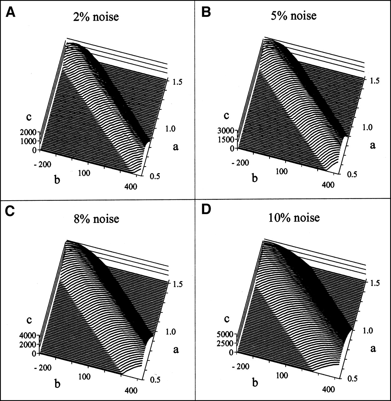
Concerning the criteria, the optimal amplitude for the noise NDSC is first discussed. Criterion maps showed a slightly noisy behavior for a low NDSC level (from 0% to 2%–3%), as illustrated in Figure 1A. Inversely, the signal-to-noise ratio in the criterion maps increased when NDSC amplitude was increased, but the full width to half maximum of the “crest” in the criterion map increased simultaneously (Figs. 1B–1D). Thus, to precisely determine the maximum criterion value, a noise amplitude of approximately 4% seemed to be a good compromise. The validity of this choice was also partly confirmed by the relative stability that was observed above a 4% noise level for the optimal parameter values, in particular for the 2-parameter model. Indeed, the noise amplitude proved to be a far less critical parameter for the 1-parameter model. The instability of the 2-parameter results was probably enhanced by the strong correlation that linked the α and β parameters. The tunnel shape of the criterion surface in Figure 1 clearly illustrates this correlation.

Representative DSC criterion maps obtained for 1 patient with different noise amplitudes: 2% (A), 5% (B), 8% (C), and 10% (D). Criterion value (c-axis) is drawn as function of α (a-axis) and β (b-axis), the 2 parameters of gray-level normalization model.
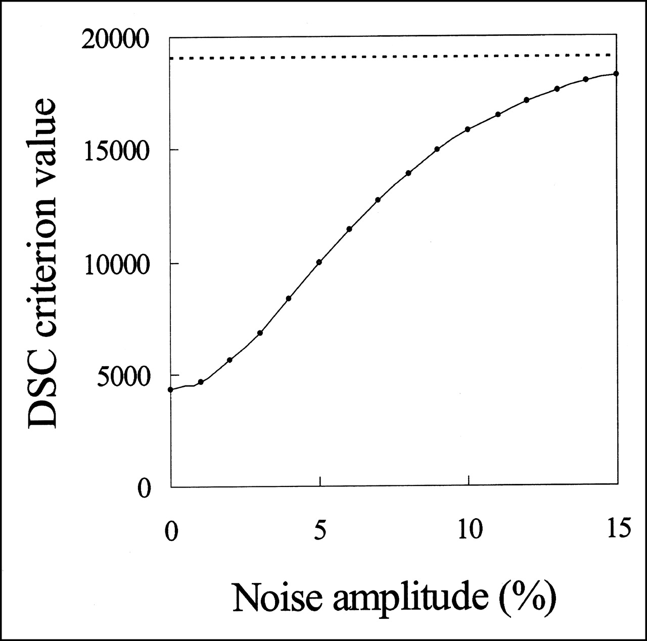
The optimal criterion value increased naturally with the NDSC amplitude: slightly between 0% and 1%; more between 1% and approximately 8%, with an inflection point near 4%; and then less and less while approaching asymptotically its maximum value. A representative curve of the DSC criterion value dependence on the NDSC amplitude is shown in Figure 2. The fact that the slope of the DSC criterion is maximal at approximately 4% may be an additional argument in favor of this value for the optimal noise.

DSC criterion value as function of noise amplitude obtained for 1 patient. Horizontal line at top (below 20,000) shows theoretic maximum criterion value, toward which criterion value should converge asymptotically with increasing noise.
We now compare the criteria. For the 1-parameter model, 4 among 5 criteria (Mean, Med, DSC-1, and Lin-1) gave very similar results (Table 5, line 1). On the contrary, the Max criterion led to α values that differed substantially from the values obtained by the other criteria (Table 5, line 2). Especially, differences reached 17% for patient 1 and 11% for patient 3. For the 2-parameter model, the Lin-2 and DSC-2 criteria gave comparable results (Table 5, line 3). The rather high α variations were mainly caused by some high values (i.e., 13% and 5% for patients 1 and 3, respectively).
Influence of Criterion and Normalization Model on Gray-Level Normalization Parameters
For the comparison of the 1- and 2-parameter models, methods Lin and DSC were considered. From the above-mentioned similarity of results between DSC-1 and Lin-1 on one side and between DSC-2 and Lin-2 on the other side, one can deduce that the differences existing between Lin-1 and Lin-2 were similar to the differences existing between DSC-1 and DSC-2, as summarized in Table 5, lines 4 and 5. Individual discrepancies > 10% are detailed in the following. One should remember that the β value equals zero for 1-parameter models. For Lin-2 versus Lin-1, α values differed by 28% for patient 1 and by 10% for patient 6, whereas β values differed by 10% for patient 1. On the other side, for DSC-2 versus DSC-1, α values differed by 33% for patient 1, whereas β values differed by 14%.
Correlation Scatterplot and Normalization Lines.
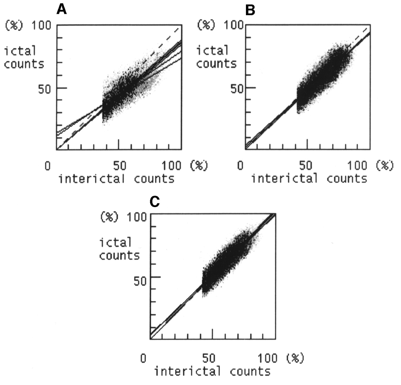
Results may be classified into 3 categories as illustrated in Figure 3. The first one (Fig. 3A) included only patient 1 and was characterized by a widely spread cluster, which probably resulted from the mixing of several subclusters. In this case, 3 groups of normalization lines could be distinguished. The Max method line obviously did not fit the correlation cluster well. Lines issued from the other 1-parameter methods and from the 2-parameter methods differed from each other; they both better fitted the correlation cluster, but neither was clearly satisfactory and it was difficult to decide which was the most valid. Even if a 2-parameter model should theoretically fit the data more tightly, the visual impression would be in favor of the 1-parameter model. The second category (Fig. 3B) included 2 patients (patients 3 and 4). In this case, a narrower cluster was correctly aligned along all normalization lines except the Max-method line, which was more or less deviated toward the upper part of the cluster. The third category (Fig. 3C) included 3 patients (patients 2, 5, and 6). In this case, the even narrower cluster was well described by all normalization lines, which were very similar to one another.

Correlation scatterplots with overlay of different normalization lines. Plots are shown from 3 representative patients, patients 1 (A), 4 (B), and 2 (C). Each voxel within reference volume is represented by a point whose coordinates are equal to interictal and ictal counts. These counts have been scaled to maximum interictal and ictal counts, respectively. Diagonal dashed line is normalization line obtained by method Max. All other lines through origin are normalization lines obtained by 1-parameter methods; the 2 lines deviating from origin are normalization lines obtained by 2-parameter methods.
Reference Images, Registered Normalized Mobile Images, and Subtraction Images Compared with Clinical Data and Other Imaging.
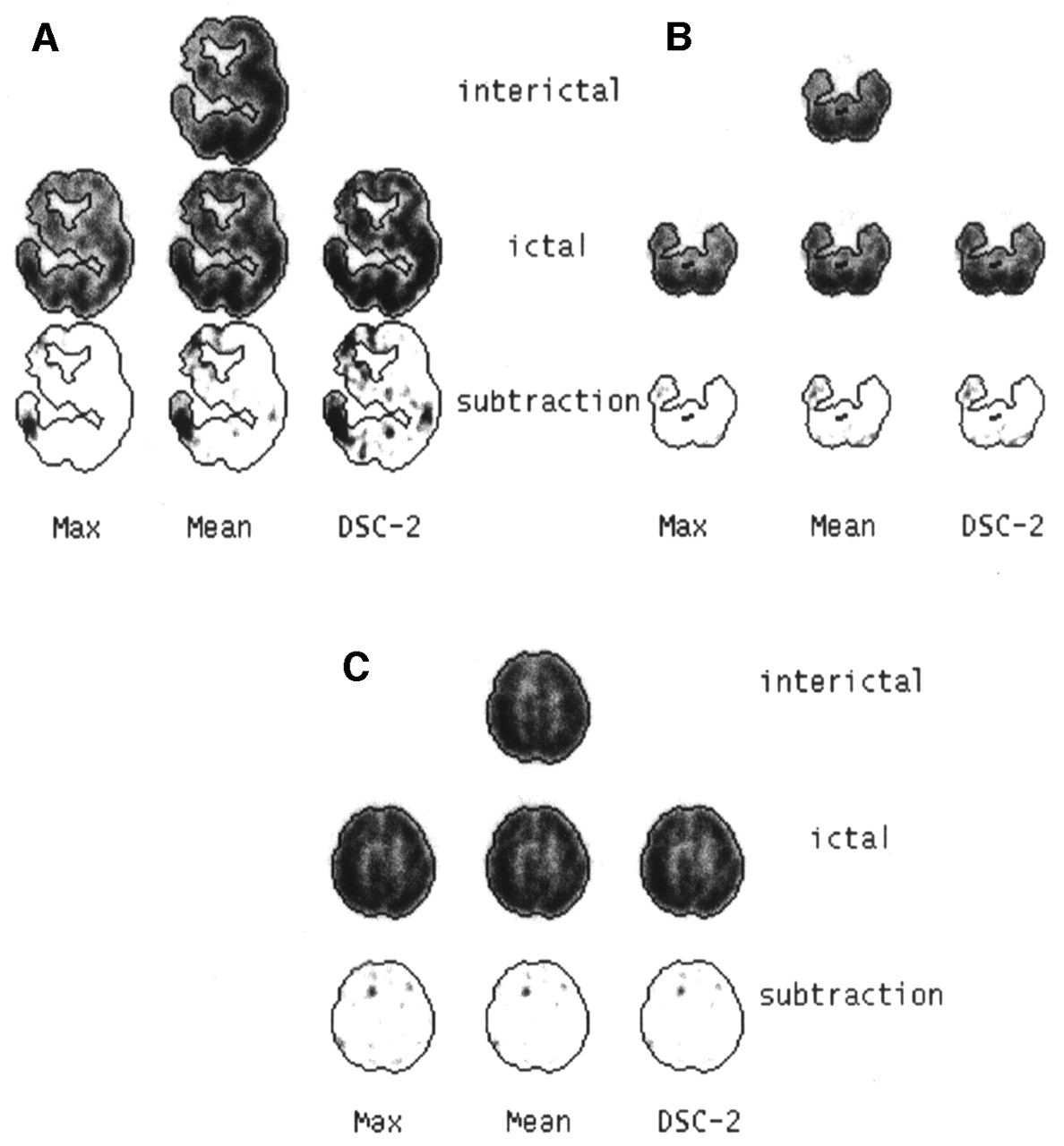
The 3 categories that were exhibited in the previous paragraph are illustrated in Figure 4. Three normalization methods representing the 3 groups of methods distinguished in the previous paragraph were chosen, that is, the Max method, another 1-parameter method (Mean), and a 2-parameter method (DSC-2).

Reference images (interictal), registered and normalized images (ictal), and corresponding subtraction images (ictal–interictal), which were obtained by 3 different normalization methods (Max, Mean, and DSC-2). Images in A, B, and C are from same patients as in Figures 3A, 3B, and 3C, respectively. Isocontours drawn from reference images are superimposed on all images. Subtraction images are saturated at 30% of maximum of reference images, but no background has been removed.
Not surprisingly, these methods differed noticeably in the first category (Fig. 4A). Normalized images were apparently either not enough saturated or too much saturated for methods Max and DSC-2, respectively. From the global visual aspect, the most satisfactory method was probably the Mean method in this particular case. Number, size, and intensity of hot spots also changed significantly in the subtraction images between the 3 classes of methods. In this case of hemispheric atrophy, extensive abnormalities were already present in the interictal state, and the whole brain seemed to be variably involved in the epileptic process; it was thus difficult to know which subtraction image better approached the clinical reality. However, clinical seizure and SPECT–MRI overlay images had shown right frontotemporal involvement, which is compatible with the findings of subtraction images obtained by all normalization methods apart from the Max method. Also, the contralateral temporal spot, which is exhibited with all methods but the Max method, is clinically plausible.
For the second category (Fig. 4B), the Max method differed to a variable degree from the other 2 methods. In the example shown here, the ictal images were slightly undersaturated for the Max method, leading, in the subtraction image, to a smaller and less intense difference in the right temporal region, when compared with the other 2 methods. Despite the consistency of ictal electroencephalography and SPECT–MRI overlay images with this temporal spot, the state of this patient (patient 4) was not improved after surgery. Other foci exhibited in the subtraction images, as well as surgical sequelae, might explain this outcome. The 2 patients of this category presented with limited abnormalities consisting of a focal area of hypoperfusion on interictal SPECT images.
For the last category (Fig. 4C), all methods gave similar normalizations and hence comparable subtraction images. In the case of patient 2, shown here, clinical seizure, electrocorticography, MR images, and SPECT–MRI overlay images gave a concordant right frontal localization, but overlay images and subtraction images showed bilateral involvement. The unilateral surgery was not successful in this patient. In patient 5, on the contrary, the right frontal focus exhibited in all subtraction images and consistent with MRI and electrocorticography was successfully cured by a right frontal lobectomy. The 3 patients of this category had interictal SPECT images visually interpreted as normal.
3D Display and VOI Analysis
An example of reference, mobile registered normalized, and difference images is displayed in Figure 5. Numeric results are given in Table 6. In the column showing the ictal-to-interictal ratios of the means in cerebellar VOIs, the ratio corresponding to method Mean deviates from 1 for patients A and C. This deviation illustrates the above-mentioned impact of the reference volume choice on normalization. As expected, the 3 types of normalization methods exhibited large discrepancies for patient A, a noticeable discrepancy between method Max and other methods for patient B, and comparable results for patient C.

Reference images (interictal), registered and normalized images (ictal), and corresponding subtraction images (ictal–interictal) for same patient as in Figures 3C and 4C are shown in 3 orthogonal planes. Isocontours delimiting cerebral VOI drawn from reference images, and contours delimiting parallelepiped target VOI, are superimposed on all images.
Comparison of Interictal and Ictal Images Using VOI Analysis
DISCUSSION
Gray-level normalization has been addressed in different contexts (6–10,16–18). Finding the optimal gray-level normalization method for comparing 2 scans from the same patient is not simple. This normalization is, however, mandatory, whatever method may be used for the comparison. In the case of epilepsy, ictal and interictal images are currently directly compared (5,19–21) and subtraction images have become a standard (9,11,18,22–26). Registration and normalization should also precede any VOI analysis, making it more accurate than if performed separately. The normalization method (reference volume, normalization criterion, and model), its validation, and some limitations are discussed below.
The reference volume choice should be driven by knowledge or at least assumptions depending on the disease under study. In the absence of precise knowledge, the chosen reference volume should probably be large enough using anatomic or statistical (18) arguments. For epilepsy, the classic choice of cerebellum is not appropriate, because of its possible involvement in the epileptic process (20,27). The contralateral lobe has been proposed for lateralized foci, whereas the cerebellum was kept as a compromise for bilateral foci (9). In our study population, the cerebellar VOI led to normalization that generally differed from whole-brain normalization. Additionally, some interoperator variability was also observed in results that issued from different cerebellar VOI choices. For other diseases, such as schizophrenia, whole brain has been reported to be a more “reliable and specific” reference than cerebellum (6).
Whole brain seems to be a satisfying choice if interictal reference images show only limited abnormalities (focal hypoperfusion or no visible abnormality), which was the case for all patients but one. The threshold value defining the brain seems to be a somewhat insensitive parameter and should, besides, not be critical if a robust similarity criterion is used. However, the validity of a global normalization method for extreme cases such as patient 1 is questionable, and hence, so also is the existence of any valid reference volume.
Concerning the normalization criterion, there were, surprisingly, no major differences between criteria with different degrees of robustness apart from the maximum, which should be discarded. Mean and median were similar, despite the a priori low robustness of the mean. The DSC criterion or its variant, the stochastic sign changes criterion, was initially proposed for the comparison of 2-dimensional scintigraphic images (28). This criterion has also been used for 3D geometric registration (29), occasionally including a normalization factor (1). But, to our knowledge, it has not yet been explicitly applied to gray-level normalization of 3D data. Results using this criterion did not differ strongly from linear regression in the cases presented here, apart from the complex case of patient 1. Other authors have used another robust criterion, that is, the minimization of entropy in the difference histogram after initialization using linear regression (25). All criteria rely on assumptions that cannot always be verified about the difference images. However, these assumptions are usually less restrictive for robust criteria.
Like the reference volume, the gray-level transformation model should be chosen from a priori knowledge (physiologic or physical) or from a posteriori knowledge (statistical and, more generally, driven by the data). In the absence of certitude, a linear model seems to be a reasonable choice. A robust implementation of a 2-parameter linear model has already been proposed for the comparison of 2-dimensional scintigraphic images using the stochastic sign changes criterion (28) and applied in different contexts, such as immunoscintigraphy or parathyroid thallium–technetium scintigraphy (30). Another robust implementation of a 2-parameter linear model, the so-called mode line, has been proposed in 2-dimensional abdominal leukocyte imaging (31). Concerning the number of parameters, the 1- and 2-parameter models sometimes led to strongly different results. Even if a 2-parameter model would fit the data more tightly a priori, we think that, if there is no physiologic or physical argument for a 2-parameter model and if the data do not support such a model, a 1-parameter model has a lower probability to artificially wrongly describe the data. Indeed, an additional degree of freedom gives the freedom to approach the truth but also to freely generate erroneous results. Arguments for choosing a simple proportional scaling, as recommended elsewhere (32), could be the simplicity of the model and the stability of the results when either the reference region threshold or the noise level for the DSC criterion was varied. This stability should be opposed to the relative instability of the results for the 2-parameter model, at least partly due to the high correlation linking these 2 parameters.
For the technical validation of registration and normalization, the 3D display and the correlation scatterplot together with the normalization line are useful tools. The correlation scatterplot contains more information than does the 1-dimensional pixel-intensity distribution of the subtraction images. Thus, the criterion sometimes used to validate a gray-level normalization—that is, the requirement that this distribution should be approximately centered on zero (23)—may probably lead to erroneous conclusions more often than does the criterion of a good visual global fit between the normalization line and the correlation cluster.
The clinical validation is particularly difficult, because differences between methods are not so important that they would lead to diverging conclusions. As long as we do not know exactly what happens in the epileptic brain, there is no reference technique to get the ground truth and consequently to know whether an apparently correct normalization is better than another normalization. A 2-y follow-up after surgery is usually recommended to draw conclusions about the actual localization of epileptogenic foci. This information was not available for each patient in this study and would not always be able to exhibit the optimal normalization method. Moreover, this study was essentially focused on the intrinsic technical comparison of different normalization methods and not on clinical validation that would require a large series of patients with a long postsurgical follow-up.
Using physical or numeric phantoms would not help one to compare methods or to assess their validity. Indeed, in this way one could test only simplified models, not models that reproduce the complexity of the unknown reality, which is the core of the problem and precisely what makes the comparison difficult.
No statistical analysis was performed. We intentionally did not average images across patients using a classic anatomic standardization (33) as was done by Lee et al. (34). We believe that such a standardization is particularly unsuited to an ictal–interictal comparison in which variable patterns of hypo- and hyperperfusion are of unknown and variable localization and affect both ictal and interictal images. With a restricted number of scans, 2 in our case, any statistical analysis at the pixel level is not applicable. This holds for parametric statistical analysis (32) and even for nonparametric statistical analysis, although the latter, like statistical analysis involving permutation, typically requires fewer assumptions (35).
We addressed only the gray-level normalization issue and did not try to assess any significant differences at a pixel or cluster level. Such a further step would require knowledge about the noise or variance in the reconstructed images. When more than 2 scans are available, either from the same patient or from different patients after anatomic standardization, noise can be estimated directly from the data. More generally, including the 2-scan case, noise can also be derived from simulations (36) or from theoretic models that have been developed for different reconstruction methods (37,38). But these noise estimations suffer from uncertainties and approximations. Moreover, applying this noise knowledge in the 2-scan case is not straightforward. Another approach could be noise suppression by some regularization procedure (39,40) that would lead to almost noise-free images and, hence, almost noise-free subtraction images.
Among possible extensions, the patient sample could be enlarged to further validate this comparison tool, especially to check that no category was missed. A clinical validation could also be performed on a large series of patients covering a wide variety of epileptic patterns. Further, it would be interesting to extend and adapt this tool to other brain pathologies (e.g., Parkinson’s disease, Alzheimer’s disease, and depression) or to other conditions (e.g., activation and drug action). This tool could also be valuably combined with available multimodality software that fuses functional images (PET, SPECT) with anatomic images (MRI, CT).
CONCLUSION
When comparing intrapatient brain SPECT images, one should be aware of the potential impact of the gray-level normalization method on clinical interpretation. Normalized and subtraction images together with numeric VOI analysis results should always be considered with care because of the sometimes unavoidable uncertainty associated with the normalization choice (reference volume, optimized criterion, number of parameters) and its consequences on the number, intensity, and size of spots in the difference images. From the results of this study, however, a simple robust scaling should be recommended for ictal–interictal images. More precisely, the classic scaling based on the mean in the brain volume seems to be a good approximation in most cases. On the contrary, scaling based on the maximum value should be discarded. Moreover, a 2-parameter gray-level normalization model is not necessary; that is, only the scaling factor needs to be determined in the linear model, with the additive constant set to zero. Only in rare cases with highly dissimilar ictal–interictal images does the question of a valid normalization remain open.
Footnotes
Received Sep. 21, 2001; revision accepted Feb. 12, 2002.
For correspondence or reprints contact: Catherine Pérault, PhD, Unité de Médecine Nucléaire et de Biophysique, Institut Jean Godinot, BP 171, 51056 Reims Cedex, France.
E-mail: catherine.perault{at}reims.fnclcc.fr


