


Abstract
Because of the limited number of projections, the mathematic reconstruction formula of the filtered backprojection (FBP) algorithm may create an artifact that streaks reconstructed images. This artifact can be imperfectly removed by replacing the ramp filter of the FBP with an ad hoc low-pass filter, the cost being the loss of contrast and definition. In this study, a solution was proposed to increase, by computational means, the number of projections to reduce the artifact at a lower cost. The cost was a postacquisition process, which was reasonably time consuming. Methods: The process was called interpolation of projections by contouring (IPC). First, level lines were plotted on the sinogram to delimit isocount regions; then, the regions containing the interpolated points were found, and to each point was assigned the intensity of its isocount region. Using this process, the data could be resampled, allowing an increase in the number of projections or the number of pixels by projections. A phantom study of bone scintigraphy was performed to compare the slices obtained with and without the IPC process with the true image. A clinical case was also presented. Results: The phantom study showed that with the IPC process, the reconstructed slice was closer to the model, inside and outside the body, when the sinogram was resampled to multiply by 2 or 3 the number of projections, with the same number of pixels per projection. In the clinical study, the streak artifact was reduced, especially outside the body, although only a ramp filter was used. Conclusion: The IPC process succeeded in reducing the streak artifact. This process did not require any modification in acquisition and was not operator dependent. The increase in the number of projections is likely a necessary but not a sufficient condition to reduce the streak artifact: if not corrected, the attenuation could be a limiting factor in the removal of this artifact when the number of projections increases.
Filtered backprojection (FBP) is a technique used in nuclear medicine and CT to reconstruct a slice from a set of its projections (1–3). The FBP technique uses a fast algorithm, but its streak artifact (or star artifact), which is present in both nuclear medicine and CT modalities, is a drawback. In nuclear medicine, this artifact is especially visible when a small region in the slice of interest contains high activity. The artifact is caused by the small number of acquired projections (in practice, usually equal to the matrix size of the slice), whereas an infinite number of projections is theoretically required to perfectly reconstruct a slice. The mathematic formula of the FBP uses a ramp filter, but usually, to reduce the streak artifact, this ramp filter is replaced by a low-pass filter. This results in a loss of contrast and resolution in the reconstructed image. If the number of projections can be increased, the streak artifact is expected to be reduced without the drawbacks of a low-pass filter.
The streak artifact has been extensively studied in CT. In this modality, the artifact is caused mainly by metallic implants (4). These implants strongly attenuate the x-rays and then result in projections with missing data. This lack of data produces artifacts similar to those observed in nuclear medicine. Several solutions have been proposed to remove the artifact, but although some methods are not applicable to nuclear medicine (e.g., using materials with low x-ray attenuation coefficients or increasing the effective x-ray energy (4)), others may be interesting because they rely on the generation of values to compensate for the lack of data (5–8). Using this approach, a solution in nuclear medicine might be to interpolate projections between each measured projection in the sinogram (the sinogram is the set of 1-dimensional projections of a given slice, placed from top to bottom in the order of acquisition). The goal of interpolation is to obtain, by computation, new values between points of measurement. However, the problem in CT is to compensate for the lack of data inside each projection line, and the proposed solutions are not well suited to our case, in which we have to find data between 2 successive projections.
From a theoretic point of view, when dealing with signal reconstruction one must verify whether the conditions of the Nyquist theorem are fulfilled, that is, one must evaluate the Nyquist frequency, which is twice the upper bound of the signal frequency spectrum. Let us take as an example a sinogram obtained from a 2-dimensional image with an isolated structure. The variable θ is defined as the angle of aprojection relative to the starting position. The Fourier transform of this sinogram has a maximum frequency (along the direction of the conjugate variable of θ) that increases with the distance from the isolated structure to the center of the field of view. The sampling angular interval must decrease accordingly. This result is general and is another way to explain the occurrence of the streak artifact in terms of violation of the Nyquist theorem. Therefore, interpolation of the sinogram amplitude along the coordinate directions is not correct unless Δθ is small enough. Our suggestion is to go around this difficulty by fixing the amplitude value. We then face the problem of sampling the contour amplitude, or expressing 1 coordinate in a function of the other, which happens not to be a rapidly varying signal. New intermediate projections can then be predicted, allowing a Δθ small enough from the viewpoint of the Nyquist theorem.
The difficulty in projection interpolation from a physical point of view is presented in Figure 1. An interpolation column by column inside the sinogram is expected to give poor results because movement of the detector to the next angle causes shifting of the projection of a pixel in the slice along the detector line (unless this pixel is at the center of rotation of the detector). A good interpolation must account for this shift. A physically correct solution (i.e., as close as possible to the measured data if a measurement was performed) is also shown in Figure 1. In this article, we present a level line–based method that interpolates well.

Illustration of problem. At top, set of 1-dimensional projections is acquired. At bottom, black, dotted, and white pixels represent pixels with high, mid, and low activity, respectively. Interpolation column by column (A) is not correct. Good result is presented in (B). Pixel size may be reduced (dashed lines) to make sure that new data do not straddle 2 of larger pixels.
Because the streak artifact is especially visible when the intensity is higher in a region than in the rest of the image, we tested our method on hip tomograms, in which the bones usually have a high intensity while the remainder of the image (soft tissues) has a low level of fixation. Our method was tested using computer simulation and clinical images.
MATERIALS AND METHODS
Principle
The sinogram can be seen, in 3-dimensional space, as a map on which each pixel is defined by its coordinates along the x- and y-axes (Fig. 1) and the altitude is the intensity of each pixel. Our proposal was to use a contour plot of the sinogram to draw level lines adequately joining points of equal intensity. Once these lines are found, they delimit regions of given altitudes (isocount regions). Given the coordinates of each new interpolated point, a simple algorithm finds the isocount region to which that point belongs; the intensity of the interpolated point is the altitude of its isocount region.
Implementation
The processing algorithm, which we call interpolation of projections by contouring (IPC), was implemented using Matlab (The MathWorks, Inc., Natick, MA), version 5.2, under the Windows95 operating system (Microsoft Corp., Redmond, WA). The contourc function of Matlab was used to determine the set of contour lines in the sinogram (Fig. 2). The number of levels equaled the number of integer values between 1 and the maximum value in the sinogram. The 1 level line was the line between the 0-count and the 1-count areas, and so on. An approximation might occur in a particular case: if a level line had to be created and no pixel had the corresponding value, the contourc function created the level line by linear interpolation of the lower and upper level lines. The contourc function returned a set of line segments. For the last interpolated projection after the last measured projection, the interpolation was performed between the last and first measured projections.

Interpolation process. Step A is determination of level lines. All pixels inside region with given pattern have same intensity. In step B, new points are at nodes of thinner grid, which is applied on level lines. Temporary points are determined as intersection of level lines with horizontal lines of new grid. They are used, line by line, to find value in pixels.
A Matlab script computed the coordinates of temporary points as floating point (noninteger) values. These temporary points were the points of intersection of the new projections (the horizontal lines of the new grid in Fig. 2) with the level lines. The program interpolated the coordinates of points of equal intensity; it did not interpolate the intensity between the points. These intersection points were not generally on the nodes of the new grid. The program found the isocount region of each new pixel of a new projection by determining the temporary points between which the new pixel was. When all pixels had a value, the temporary points were removed. The aim, starting from the measured (p × n) sinogram grid, was to create a new user-defined thinner (P × N) sinogram, in which p and P were the number of projections and n and N were the number of pixels per projection in the measured and new sinograms, respectively. No particular relationship between p and P or between n and N was required.
A color map was specifically designed, modifying a standard color map available with Odyssey VP workstations (Marconi Medical Systems, Cleveland OH). The first color (corresponding to 0 count), which was normally black, was here white. The rationale for this modification was to enhance the contrast of the low non-null areas and, in particular, of the streak artifacts, which were the objects of interest. No window or level adjustments were performed on the images; that is, the white color of the background corresponded to 0 count only.
For both phantom and clinical studies, 3 sinograms were created from the measured sinograms using various parameters. Table 1 presents the parameters used for interpolation and reconstruction. In case A, the transverse image was reconstructed using an unprocessed raw sinogram (120 projections with 128 pixels per projection). In cases B and C, 240 and 360 projections, respectively, were created by interpolation, with 128 pixels per projection. In case D, 240 projections were created, with 256 pixels per projection.
Interpolation and Reconstruction Parameters
Phantom Study
The IPC process was first tested on a simplified transverse slice showing a bone metastasis in the hips (Fig. 3). This image was numerically created on the computer. The activities in the regions were averages of measurements made on images of 10 patients. The body limit was the dark blue ellipsoid. The pixel value outside the body was 0 count. The image had a high definition (768 × 768 pixels), to approach reality. Using a custom Matlab projection program, 120 projections measuring 128 × 128 pixels were created. No tissue attenuation or collimator blurring was considered. Poisson and gaussian noises were added to the projections to account for the random nature of the radioactive disintegrations and the noise introduced by the imaging system, respectively. Custom programs generated random values for each pixel using the random-number generator of the computer. The maximum pixel intensity in the phantom image before noise addition was 255 counts. The Poisson noise was first added, as a function of the pixel intensity. The gaussian noise was added equally to all pixels, independently of their intensity. This noise had a mean value of 0 (i.e., negative values of noise could be generated). The SD of the gaussian noise was empirically estimated to 6 counts per pixel. Pixels with negative values were set to 0 count. Because only integer values had physical meanings, the floating values returned by the noise generator programs were rounded to the nearest integer.

Phantom (768 × 768 pixels) used as model. This image is used to generate projections for phantom study.
Clinical Study
The clinical images were of a 49-y-old man who received a bolus injection of 99mTc-methylene diphosphonate. The tomographic acquisition was performed on a Prism 2000XP gamma camera using low-energy, high-resolution parallel collimators, 3 h after injection. One hundred twenty 128 × 128 projections were acquired over 360°; that is, the angle between 2 successive projections was 3°. Each projection lasted 20 s. Figure 4 illustrates the level line image and the interpolated sinogram obtained from a raw sinogram of this bone tomogram. In this sinogram, which had a maximum pixel value of 68 counts, the contourc function found 8561 level lines, with a mean length of 9 line segments (range, 3–1024 segments).
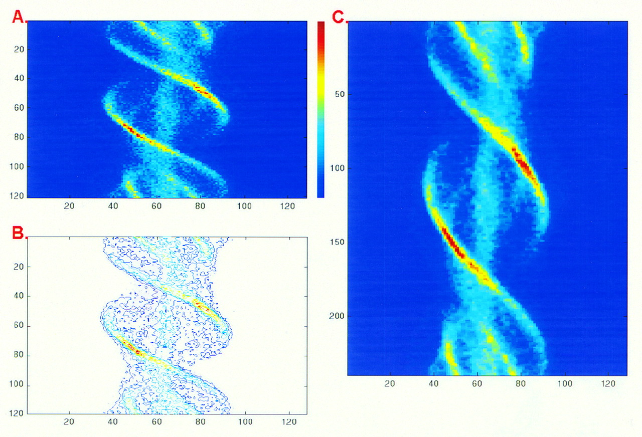
Illustration of IPC process. (A) Program input: sinogram with 120 projections. (B) Some level lines obtained from sinogram using Matlab contourc function. (C) Program output: sinogram used as input, now with 240 projections.
Image Reconstruction
All transverse images were obtained using the commercial FBP program available on our Odyssey VP workstation (Marconi). In all cases, no pre- or postreconstruction filter was used, only the mandatory ramp filter.
Image Analysis
For the phantom study, the transverse images obtained from raw and interpolated sinograms were compared with the model. Because they had different matrix sizes, the transverse images were converted to images with 768 × 768 pixels (the size of our model), by mapping the 128 × 128 or 256 × 256 images. The differences between the model and the transverse images were assessed separately inside and outside the body, using the index d defined as:
 Eq. 1where Nmodel was the number of pixels of the model inside or outside the body (inside: 180,124 pixels; outside: 409,700 pixels).
Model(i,j) and reconstructed(i,j) were, respectively, the pixel values in the model and reconstructed images, inside or outside the body. If, for a given pixel, the value in both the model and the reconstructed images was null, the ratio in Equation 1 was set to 0. This index was a simple, dimensionless variable that gave relative improvement. For the clinical study, the artifact was quantitatively estimated by the number of non-null pixels outside the body and the sum of their values.
In this article, the raw transverse images refer to the transverse images obtained with acquired projections only, and the processed images refer to the transverse images reconstructed from the projections obtained after the IPC process.
RESULTS
Phantom Study
Without noise (Fig. 5), the raw transverse image exhibited a streak artifact that originated mainly from the hot spot mimicking a metastasis. The artifact was visible inside and outside the body. After the IPC process, when the number of projections was 2 or 3 times the number of measured projections, this artifact almost disappeared outside the body and was dramatically reduced inside the body. The reconstruction with 240 or 360 projections gave similar results. These observations were consistent with the quantitative results, which were the values of the index d (Table 2). The 256 × 256 image obtained with 240 projections showed a very good reduction of the streak artifact outside the body, but this artifact was still clearly visible inside the body; the quantitative analysis confirmed that, compared with the raw image, no improvement occurred inside the body.

(A–D) Transverse phantom image obtained for 4 cases described in Table 1, when no noise is added to projections. Each image is normalized to its own maximum; minimum value of window value is 0, and no window or level adjustments or similar operations are performed.
Difference Between Reconstructed Images and Model
With noise, the radial streaks clearly visible in the raw image (Fig. 6A) were not present in cases B and C and were reduced in case D. The difference inside the body between the images and the model were reduced when the number of projections increased (Table 2), but, as it was the case when no noise was added, no clear improvement inside the body could be evidenced when the matrix size was 256 × 256 (case D). The difference between the model and the reconstructed images was greater with noise than without noise, except inside the body in cases A and D.

(A–D) Transverse phantom image obtained for 4 cases described in Table 1, when Poisson and gaussian noises are added to projections. Each image is normalized to its own maximum; minimum value of window value is 0, and no window or level adjustments or similar operations are performed.
Clinical Study
The radial streaks on the bone scintigram (Fig. 7) appeared to be reduced in cases B and C, but the difference was not clear in case D. Quantitatively, the number of non-null pixels outside the body and the sum of their values in cases B and C were less than half the same indices estimated in case A (Table 3). In case D, the number of non-null pixels was lower than in case A (the difference in matrix size was considered by dividing the number of pixels in case D by 4).
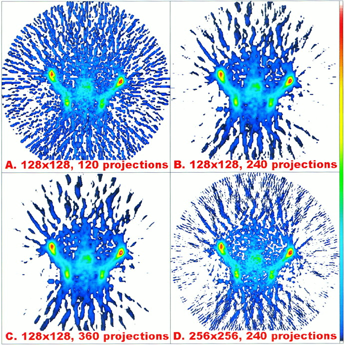
(A–D) Transverse clinical image obtained for 4 cases described in Table 1. Each image is normalized to its own maximum; minimum value of window value is 0, and no window or level adjustments or similar operations are performed.
Non-Null Pixels Outside Body in Clinical Study
DISCUSSION
In this study, we proposed a solution to increase the number of projections without increasing the acquisition time. New projections are created after the acquisition process, by interpolation of the measured projections. The interpolation does not increase the amount of information but is well suited to reduce the streak artifacts that decrease the quality of tomographic images reconstructed by FBP when some regions with high activity are present.
For several years, iterative algorithms have competed with FBP for routine use. One of the arguments in their favor is that the streak artifact does not occur or is markedly reduced when using them (9). However, we show that the streak artifact can also be reduced with FBP. Another argument in disfavor of FBP is the difficulty in choosing the nature and the features of the smoothing filter (e.g., Hanning or Butterworth) usually required to reduce the streak artifact; no such filters are used in this study, and the mandatory ramp filtering has no parameters (especially no cutoff frequency).
Our approach based on the determination of level lines theoretically permits good interpolation, as presented in Figure 1. The quality of the interpolation process does not depend on the complexity of the sinogram or on the activity level, that is, the low- and high-activity regions in the sinogram are equally processed. Moreover, the sinogram is seen as a map and no biophysical significance is under consideration; in particular, no difference is considered in the processing of regions with a low or high signal-to-noise ratio. The IPC process appears to slightly smooth the transverse image (Fig. 7), and this smoothing is likely caused by the approximations performed during the level line determination, as evoked in the implementation section of the Materials and Methods.
One reasonable hypothesis was made in this study: we assumed that the level lines could be defined by sets of linear segments. This hypothesis was assumed to be valid as long as the angle between 2 successive projections is small, and this is so when 120 projections are acquired over 360 degrees.
The IPC process is operator independent; in particular, it does not require manual or semiautomatic determination of the contours proposed to eliminate streak artifacts in CT (10). The processing time is approximately 100 s to interpolate 120 projections with 128 pixels each, using a personal computer with a 333-MHz microprocessor; the time should be markedly reduced for software written in C instead of Matlab functions and scripts.
The phantom and clinical images are not improved by the IPC process when the reconstruction matrix is 256 × 256 pixels and the sinogram has 240 projections. This result is consistent with the notion that to optimize reconstruction, the number of projections must increase as the matrix size of the slice increases: Huesman (11) recommends that the number of projections be equal to 1.5 times the number of the matrix size of the reconstructed slice for an optimal reconstruction (e.g., for a 128 × 128 slice, the number of projections acquired should be 192 [128 × 1.5]). This condition is verified when a 128 × 128 slice is reconstructed from 240 projections but not when a 256 × 256 slice is reconstructed. For the latter, 384 projections (256 × 1.5) would be required according to Huesman.
In CT, the strong attenuation of metallic implants is responsible for streak artifacts (4). In our clinical study, streaks could be similarly generated because no attenuation correction was performed, and this factor could explain why the streak artifact was less efficiently reduced in the clinical study than in the phantom study, independently of the number of projections.
Usually, a low-pass filter (such as the Butterworth filter) is used with the ramp filter to reduce the streak artifact. Reducing this artifact using our IPC process allowed the reduction of such low-pass smoothing. This result, combined with the possibility of reconstructing the slice with a higher matrix size (because the number of projections and the number of pixels per projection increase), should permit better resolution with the same noise level, and this hypothesis is currently under investigation in our laboratory.
CONCLUSION
The IPC process can reduce the streak artifact without any change in the acquisition protocol by increasing the number of projections using a postacquisition process. The potential uses of the IPC process are not limited to this application, and we are studying others: the number of measured projections could be reduced to half, and the IPC process could be used to compute other projections; thus, the acquisition time could be divided by 2 at a cost of a reasonable decrease in image quality. The IPC process could also be used to detect and to replace a measured projection by a computed projection, if the measured projection is corrupted, particularly if a patient moves during a projection. Another potential use can be to increase the number of pixels and, consequently, to reduce their size before zooming an image.
Footnotes
Received Aug. 27, 1999; revision accepted Mar. 28, 2000.
For correspondence or reprints contact: Philippe P. Bruyant, PhD, Biophysics Laboratory 8, Avenue Rockefeller, 69373 Lyon Cedex 08, France.


