HOME HELP FEEDBACK SUBSCRIPTIONS ARCHIVE SEARCH TABLE OF CONTENTS		QUICK SEARCH:   [advanced] Author: Keyword(s): Year:  Vol:  Page:

This Article Abstract Figures Only Full Text (PDF) Alert me when this article is cited Alert me if a correction is posted Services Email this article to a friend Similar articles in this journal Alert me to new issues of the journal Download to citation manager Citing Articles Citing Articles via HighWire Citing Articles via Google Scholar Google Scholar Articles by Thie, J. A. Articles by Smith, G. T. Search for Related Content PubMed Articles by Thie, J. A. Articles by Smith, G. T.

The Diagnostic Utility of the Lognormal Behavior of PET Standardized Uptake Values in Tumors

Department of Radiology, Biomedical Imaging Center, The University of Tennessee Medical Center at Knoxville, Knoxville, Tennessee

	ABSTRACT

TOP ABSTRACT INTRODUCTION MATERIALS AND METHODS RESULTS DISCUSSION CONCLUSION APPENDIX REFERENCES

 
A meta-analysis of data primarily from PET oncologic investigations using FDG PET was performed. Its purpose was to establish statistical features of the distributions of standardized uptake values (SUVs) as possible aids in the diagnostic process. Methods: We obtained 1536 values of oncologic markers from patient studies of 40 investigations in the literature. Statistical parameters were tabulated for analysis. Results: A significant observation is that, unlike skewed SUV histograms, log₁₀SUV has Gaussian behavior, which is not uncommon for biologic quantities. This was found for SUVs of FDG and 2 amino acids as well as a few other cancer markers. A possible model for explaining this is proposed. For FDG, the SD of the log₁₀SUVs for an average cancer category was 0.23. Examining data within the framework of the model points to physiologic factors as dominating SUV variability rather than PET protocols. When data for a single cancer category were available from multiple institutions, averages, s, disagree beyond chance expectations. Diagnostic utility suggestions include a universal linear relationship between sensitivity and severity, defined as SUV/, on semilogarithmic probability paper; a generic receiver-operating-characteristic curve for all cancers; using [log₁₀(_mal/_norm)] ÷ (_mal² + _norm²)^1/2 as a simple diagnostic effectiveness measure; and using Gaussian log₁₀SUVs to avoid erroneous P values. Conclusion: Using the logarithms of markers, such as SUVs, several advantages stemming from their Gaussian nature can be achieved with benefits ensuing to the diagnostic process.

Key Words: FDG • cancer • statistical analysis • standardized uptake value • PET

	INTRODUCTION

TOP ABSTRACT INTRODUCTION MATERIALS AND METHODS RESULTS DISCUSSION CONCLUSION APPENDIX REFERENCES

 
Presently, FDG is the most popular tracer in PET oncology. This stems from tumor metabolism being characterized by enhanced glycolysis compared with normal or benign tissue. A frequently used quantitative aid is the standardized uptake value (SUV), which is basically the ratio of 2 specific activities: that of a tumor at the study's end and a temporally constant entire body average. Its clinical appeal, compared with various other quantitative approaches, lies in its simplicity. Thus, the SUV is very commonly used as an adjunct to visual interpretations. Not surprisingly, an overwhelming volume of SUV data has accrued in PET oncologic literature.

An underlying premise of this investigation is that the application of statistical information contained in SUV data might improve diagnostic usage of the latter. Statistical models have been applied (1–3) to cerebral glucose metabolism and blood flow with analogous motives. That oncologic diagnostic methods might benefit from a statistical study of SUVs stems from a basic principle that the mean values, s, and shapes of overlapping benign or normal and malignant SUV distributions (i.e., histograms) directly determine a study's sensitivity and specificity (4). The ± SD is universally reported for patient subgroups. However, research on distribution shape and its influences on the underlying performance of the FDG protocol is essentially nonexistent. A rare exception is the research of Ponto et al. (5), who showed histograms of normal liver, spinal vertebrae, and thyroid FDG SUVs; however, those data were summarized as means ± SD for further use. An investigator, recognizing that the SUVs skew toward high values, might, on rare occasions, report a median rather than a mean. However, the consequences of this shape have been ignored. In t testing, ANOVA, Pearson correlations, and so forth, failure to recognize the skewed distributions that violate Gaussian assumptions can possibly lead to incorrect conclusions.

Besides documenting SUV distribution features extracted from data in FDG literature, we have searched for practical applications of these in diagnoses and for insights offered: These include addressing underlying phenomena responsible for distribution features. This has yet to be confronted even though reducing distribution widths (i.e., data variabilities) would have an immediate payoff in terms of improved sensitivity and specificity.

In many facets of biology, research has been directed toward statistical distributions. A not uncommon result in many investigations came from the logarithms of observable biologic quantities. These, rather than the quantities themselves, exhibited nature's ever-prevailing Gaussian (or normal) histogram shape (6). Prominent among explanations for this is the law of proportionate effects involving randomness in multiplicative factors occurring in a process (Appendix). A few examples of lognormal behavior among numerous ones in the literature are doubling times of cancers, sizes and weights of species, sensitivities to drugs, tumor sizes, and cell geometric quantities including cell density in tumors. Taking this cue from others, our work therefore examines the consequences of hypothesizing a lognormal distribution for the SUVs—that is, testing log₁₀SUV data for a Gaussian shape.

	MATERIALS AND METHODS

TOP ABSTRACT INTRODUCTION MATERIALS AND METHODS RESULTS DISCUSSION CONCLUSION APPENDIX REFERENCES

 
A well-planned, multicenter prospective investigation would be the ideal approach for obtaining the SUV data. However, many patients would be required. Therefore, as an initial exploration that can give immediate results, a compromise approach was to use meta-analysis (7). With this technique, SUV distribution data were examined retrospectively in each of many separate historical investigations. Its limitations must be recognized (8). For example, discussions of patient population characteristics below point out some issues.

An oncology database that was created required defining acceptance criteria. The database emphasized primarily the SUVs of malignant lesions in FDG PET. It sought variety in cancer categories and institutions studying these, provided there were sufficient numbers of lesions in each investigation:

• From an investigation, n 20 lesion or normal tissue quantifiers, with these obtained from a minimum of 13 (human) patients
  
• Reported individual quantifier values identifiable in a tabulation or graph
  
• Exclusion of studies that monitor the effects of treatment
  
• Investigations appearing in English language publications since 1987
  
• Accepting the investigator's defined patient population and classification of cancer studies, but not having metastases from a particular type mixed into a category having other types. The investigator's policy on whether to exclude diabetics was also accepted.
  

Most investigations included scans of only untreated patients. Otherwise, months between treatment and scanning would be typical. Ideally, classifications might be based on the many discrete classes from histology. Unfortunately, if these were used the number of available published investigations would be substantially reduced, and this would often lead to subgroups having too few patients for statistical analyses. Hence, cancer classifications of investigators were adopted here.

For purposes of some limited comparison with FDG SUVs, data from 2 amino acid PET tracers as well as cancer markers from CT, tumor volume, and DNA were included. The SUVs from a few investigations of normal tissues were also examined. Unfortunately, publication bias (investigators more prone to publish tumor data) discriminates against having more normal tissues represented.

For each investigation, there was a tabulation of its quantitative marker—usually SUV—with the postinjection time for its evaluation noted. These markers provided the input information to spreadsheet (Lotus 1-2-3. Cambridge, MA: Lotus Development Corp.; 1989) and statistical (Statistica. Tulsa, OK: StatSoft, Inc.; 1997) software. Only in one sixth of the PET investigations were there corrections involving the partial-volume effect, plasma glucose concentration, and body fat content. One fifth of the FDG investigations were conducted with diabetics excluded; in all others, only a few cases of abnormally high glucose were reported.

Popular quantifiers of distributions were calculated. Other specific statistical measures were Lilliefors implementation of the Kolmogorov-Smirnov goodness-of-fit test for Gaussian behavior, Kruskal-Wallis analysis of variance by ranks, and Bartlett's test for equality of variances.

	RESULTS

TOP ABSTRACT INTRODUCTION MATERIALS AND METHODS RESULTS DISCUSSION CONCLUSION APPENDIX REFERENCES

 
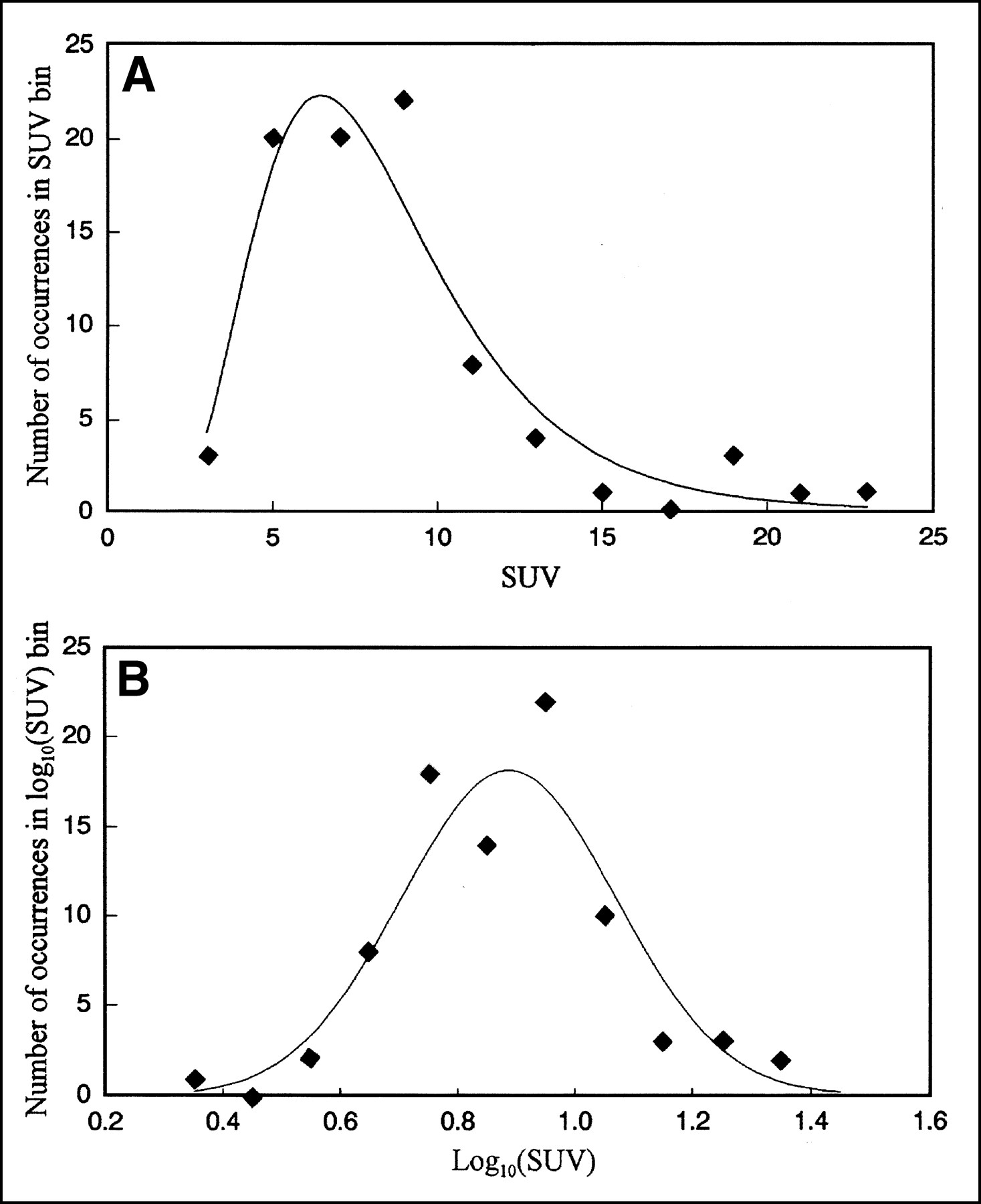
Using the SUV data of Delbeke et al. (9) as typical, Figure 1 shows the tendency of the histogram to be positively skewed (i.e., toward higher values). Such histograms are characterized by 3 parameters: mean, SD, and skew (Appendix, skew formulae). On the other hand, the log₁₀SUV histogram of these data is symmetric and would be well characterized by just SD and mean. Tables 1 and 2 summarize the statistical findings of this meta-analysis. For example, the data of Figure 1 were used in calculations for one of the rows in Table 1. A result showing indications of how logarithms reduce and remove the positive skew may be found in the columns of skew ÷ its measurement SE. The 2.9 average of this quantity for SUVs from 25 FDG tumor investigations was rather high; the average was only 0.3 for log₁₀SUVs.

View larger version (18K): [in this window] [in a new window]   FIGURE 1. Histograms of 83 metastatic liver lesions from Delbeke et al. (9) as representative. Highly skewed FDG SUV distribution (A) becomes Gaussian when its logarithm is used (B). Mean and of latter are 0.89 and 0.18, respectively, from Table 1.

View larger version (20K): [in this window] [in a new window]   FIGURE 2. Diagnostic sensitivity for 921 malignant lesions from 25 FDG investigations of various cancer categories. Commonality seen here stems from Gaussian probability axis used in combination with severity, SUV/, expressed on logarithmic scale. Slope of fitting line is related to average 0.23 SD of log10SUVs for all cancer types in Table 1.

In 4 of the FDG investigations the average number of lesions per patient exceeds 1.5. As 1 type of assessment of any multiple lesion effect, where data were available, calculations were also performed with a patient's multiple lesions replaced by just a single lesion with an average SUV. In no instance did this have more than a 1.05 factor effect on an investigation's CV.

The average time of evaluations for FDG SUVs in tumor studies was 57 min, with a SD of 8.5 min. This leads to variability associated with the rising SUV(t). Results of a simple theory (10), based on population SUV(t) of several cancers, gives (d[SUV]/dt)_{57 min} x (8.5 min)/(average SUV) 0.035. This, on average, is the small CV effect attributable to ±8.5-min evaluation time variations.

Other data at the bottom of Table 1 and in Table 2 supplement that of FDG SUVs for tumors. These data also exhibited lognormal behavior. This tends to suggest a wide occurrence of this distribution among markers. The few data from modalities other than PET, with considerable variety in their methods and tissues, showed more scatter in the values tabulated—that is, more than the 0.11–0.32 range from FDG SUVs in tumors.

	DISCUSSION

TOP ABSTRACT INTRODUCTION MATERIALS AND METHODS RESULTS DISCUSSION CONCLUSION APPENDIX REFERENCES

 
Data Features
Many investigations have taken place encompassing various cancer categories and involving the popular FDG tracer of PET. A small subset of these met our criteria for inclusion in Table 1. For this subset, additional distribution characteristics of results—especially information beyond the ± SD typically reported—have been calculated from published data.

A somewhat subjective ranking, in a decreasing importance order, for a distribution might be the mean, SD, and skew. The CVs are preferred to SUV SDs. Being normalized, the CVs' range of values among cancer categories was consequently more restricted than that of wide-ranging SUV SDs. Similarly, a more-or-less restricted range was found for the log₁₀SUVs' , as the latter is essentially the SUV CV ÷ 2.303 (Appendix). Nevertheless, statistical testing showed no commonality among s of the different cancer types.

Tables 1 and 2 show that the logarithm operation on SUVs tended on average to remove skew. Moreover, the small positive and negative skews were equally likely for log₁₀SUV. On the other hand, SUV distributions always showed positive skews. For log₁₀SUVs, the largest ratio of skew to its SE found in a total of 40 investigations in Tables 1 and 2 was only 2.3. This skew removal is associated with the functional nature of taking a logarithm: compressing values, with larger ones causing the skew in SUVs being compressed more.

The global cerebral glucose metabolic rate is not in Table 1 because it is well reviewed elsewhere (11,12). This is closely related to the SUV. Thus, its statistical behavior might be compared with findings from Table 1. A review by Wang et al. (11) provided data for compiling Table 3: The data from multiple investigations of normal brain tissue were examined further in the manner of Table 1. Normal brain tissue shows a significantly smaller FDG than all tumor types. The many factors influencing cerebral glucose uptake have been well studied and understood (11,12). Presumably aware of and accounting for these, investigators have been able to obtain a more-or-less intrinsic constancy in brain tissues' uptake in a well-defined population. Also, for both cancers and normal brain, the spread of the s is about twice that expected from a hypothetic circumstance of all investigations assumed to have the same intrinsic variance of their s. This corroborates Bartlett's test result, which indicated a lack of homogeneity among categories in Table 1.

Theoretic Reasons for Lognormal Distribution
Gaussian distributions fitting log₁₀SUVs is a significant observation. A variable with this type of distribution that is found so frequently in nature might be regarded as a more natural marker than a distribution that is non-Gaussian. However, because of limitations from available numbers of lesions or patients for a distribution, it has not been uniquely determined that the logarithm, rather than some other function, is best. Hence, the empiric evidence favoring logarithmic usage might be supplemented with some theoretic points.

There are underlying factors responsible for observed SUV variabilities in a given institution's investigation of a single cancer category, using the individual locally standardized procedures. A review by Carson (15) shows that these factors are attributed to separate influences: fundamental physiologic, test measurement, and data analysis. One approach is to express the observed SUV approximately as a product of factors, all of which contain their own internal sources of variability. This extends and quantifies a proposal by Bland and Altman (16) that rate constant products can lead to lognormal distributions:

The first factor is the Gjedde-Patlak accumulation rate K. It and the second factor approximate the patient's intrinsic SUV in terms of basic physiologic quantities (17). Equation 1 contains the rate constants of the model of Sokoloff et al. (18). Here the product, PS, of capillary permeability P and its surface area per gram S is an explicit replacement of this model's rate constant k₁. V is an entire body distribution volume associated with a tracer plasma clearance rate k_p.

The PET protocol factor is a calibration factor, defined as the ratio of measured SUV to intrinsic SUV. It is the product of many (measured ÷ true) factors originating from many variability sources (1,12–14). These include counting statistics and corrections not fully made in interpreting the SUV measuring process. In particular, the absence of any partial-volume correction is a source of variability, with substantially different results possible from scanners of different resolutions, as shown by Grady (19).

Explaining the magnitude and shape of an observed SUV distribution would require a rigorous quantitative examination of individual statistical distributions of every variable component in Equation 1. However, the scope here is limited to commenting on the possible dominant causes of variability. The relative importance of protocol versus physiologic factors might be judged from the following:

• In studying lung cancer, Minn et al. (20) found excellent FDG PET reproducibility in the same patient, obtaining CVs for SUVs and glucose-corrected SUV-leans (i.e., calculated from lean body mass not total body weight) of only 0.1 and 0.06, respectively. Similarly, for a variety of malignancies, Weber et al. (21) found the same patient reproducibility with a 0.09 CV for SUVs.
  
• Many investigations of the cerebral glucose metabolic rate (11,12) typically show CVs as low as 0.19 (Table 3), which includes both patient and PET effects.
  
• Table 4 from the work of Avril et al. (22), showing possible SUV definitions, illustrates variations from this source. These are responsible for, at most, a CV associated with methods of about the 0.20–0.22 shown in the last row of Table 4.
  

With data showing the left side of Equation 1 to be lognormal, the product of the first 2 (dominating the variability) explanatory factors on the right must now be lognormal. If variations in individual subfactors in these are lognormal, then a mathematic consequence is that the entire combination is lognormal. It is tempting to theorize perhaps a variability dominance from the vascular surface area per gram S: in a specific tissue (as a factor in k₁) and in all body tissues (as a factor in k_p). This is because it is well established (23,24) that morphologic aspects of vasculature have lognormal distributions. Also corroborating the ideas are in vitro data from an ovarian carcinoma cell line (25): FDG uptake was proportional to cell density, whose distribution is lognormal (6) and relates to S.

The range noted for the CVs or s of FDG among malignancies can also be discussed within the context of Equation 1. From Bartlett's test result, ranging was wider than would be expected if all cancers had the same intrinsic CV. However, the test showed that this range, 0.11–0.32 for in Table 1, was not excessively large for 25 investigations. Some insight might come from isoleucine uptake (26) in normal rat brain as a well-defined tissue type: CVs remaining essentially constant in spite of PS values being made, by concentration changes, to span a factor of 200. Perhaps in line with this, diverse cancer categories, with no doubt widely varying PS values, might be expected to have at least not a drastically wide range of CVs.

Potential Applications in Diagnoses
Considering our results and the above discussion, specific applications in the diagnostic process arise.

Quality Assurance.
Checks are desirable for a new tracer investigation or for an institution initiating PET studies in a particular category. With sufficient patient and lesion numbers (perhaps 20 or more), multiple comparisons with row values in Tables 1 and 2 can provide stringent tests for the newer work. This testing is whether it is within expectations relating to means and CVs measured in prior investigations.

Outliers and P Values.
Advantages of transforming data to a Gaussian variable to facilitate statistical testing have been discussed by Bland and Altman (16). One reason for doing this is to permit the use of parametric tests that require Gaussian behavior. Such tests have more statistical power (i.e., use fewer patients or reduce chances of error in conclusions [or both]). This contrasts with the required use of less powerful nonparametric tests on skewed SUVs. Some instances in which investigators have tested skewed SUV data, rather than Gaussian log₁₀SUVs, using parametric methods are now known to be incorrect; false conclusions could have resulted possibly from erroneous P values. It is easy to appreciate that forcing an assumed Gaussian shape on a skewed distribution such as Figure 1A can lead to a very poor representation of the tails, which influence statistical decision making.

Receiver-Operating-Characteristic Curves.
Receiver-operating-characteristic (ROC) curves now can be constructed more accurately over wider ranges with fewer patient data. After transforming SUVs to log₁₀SUVs, a 2-parameter fit to a Gaussian distribution is possible. This provides a basis for extrapolations into distribution tails beyond data. If need be, it is even possible with limited data to use historical information on . This would permit approximating a distribution when only its measured mean is available. Once the best distribution curves for available numbers of patients for both malignant and benign or normal categories are gotten, the construction of an ROC is straightforward (Appendix).

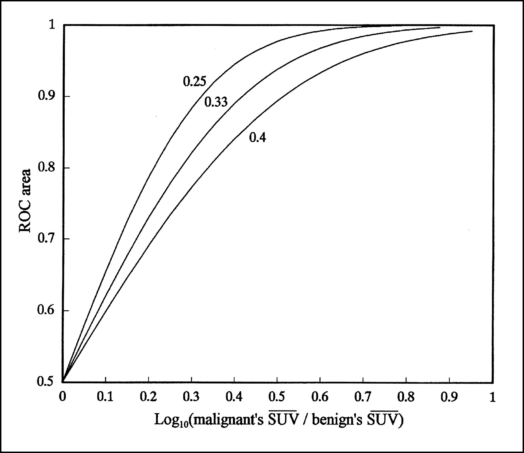
Figure 3 illustrates generic ROCs on double probability paper (Appendix). Noteworthy is its primary dependency on only a ratio of s. Secondarily, there is also a dependence that is not shown because this ROC uses its generic 0.23 value for both malignant and benign or normal distributions.

View larger version (51K): [in this window] [in a new window]   FIGURE 3. Generic ROCs for use in approximately describing any cancer category. Parameter shown identifying line is log10(mal/ben), where subscripts indicate malignant and benign, respectively. Better straight-line descriptions are possible, provided there is sufficient number of patients. These would improve on 0.23 used for SDs of both malignant and normal log10SUVs in calculations here.

Test Figure of Merit.
The diagnostic capabilities of 2 tests having lognormal test values x, such as SUVs, may be compared using a simple figure of merit (FOM). Suggested is (Appendix, geometric mean usage)

(Eq. 2)

where

(Eq. 3)

may be used to characterize test effectiveness. The larger the FOM, the larger the ROC area, which, using the probability function (Appendix), is (FOM). Figure 4 shows this function. When lacking better information, the _t may be approximated with an average over all tissue types, (0.23² + 0.23²)^1/2 = 0.33, based on Tables 1 and 2.

View larger version (19K): [in this window] [in a new window]   FIGURE 4. ROC area for comparing tumor diagnostic protocols. Parameters identifying these lines are total SDs—that is, square root of sum of squares of s belonging to benign and malignant log10SUV distributions. For central line, its (0.232 + 0.232)1/2 = 0.33 is typical t of cancer categories of investigations here.

Interinstitutional Comparisons.
Keyes (14) has critically questioned the use of published SUVs outside an investigator's institution. As discussed above, when there were 3 or more investigations of the same cancer category (which often included various histopathologic types), the results were significantly different. It would be especially inappropriate for an institution to blindly use a (benign versus malignant) cutoff SUV recommended by another institution. This is because of a need to thoroughly compare protocols and makeups of patient populations and to agree with outcomes' cost–utility assignments explicitly or implicitly made in optimizing cutoff.

Until standardized approaches are adopted, the options in Table 4 and other protocol variations known to affect SUVs should be recognized (1,12–14). Sometimes a choice of a best SUV definition is recommended for a given tissue, as in the work of Avril et al. (22). For the present, the practice of an author attaching a designator to the SUV acronym is commendable, though rare. As an example, SUV_avl(55) would indicate average pixel values, lean body mass, and 55 min after injection.

It is also important to heed proper characterizations of patient populations. From the discussion of Equation 1, patient factors, rather than PET factors, are implied as the more important contributors to SUV variability. Noted in the discussion of Table 3 was identification of patient factors (11,12) as helpful in reducing CVs of cerebral glucose metabolic rates. One step in this direction in oncology is the often-seen listing of SUVs with the histopathology, along with other descriptive disclosures.

SUV Ratios, CVs, and Geometric Means.
These quantities arise out of relationships from usage of logarithms (Appendix) and are intrinsically more appropriate to use than SUV differences, SDs, and arithmetic means. In particular, in light of Figure 2, the use of severity, as SUV ÷ a population's , departing from unity is a universal measure that is independent of cancer type.

	CONCLUSION

TOP ABSTRACT INTRODUCTION MATERIALS AND METHODS RESULTS DISCUSSION CONCLUSION APPENDIX REFERENCES

 
This work should bring out an awareness of an inherent logarithmic and multiplicative nature of tracer uptake. Distribution data supporting this are convincing. It is encouraging to note this commonality of a Gaussian distribution of log₁₀SUVs of all cancer and other tissue categories with many other lognormally distributed quantities in biology. On the other hand, more work is needed for a quantitative understanding of a possible explanatory law of proportional effects unfolding in tracer uptake at the cellular level.

On the basis of our findings, several practical diagnostic aids are suggested. These lead to a belief that benefits in information portability among institutions could result from steps taken in at least 2 directions: standardizations of PET protocols along lines of reducing variabilities and more attention to detail regarding factors within a cancer category population that might influence individual SUVs. Narrowly defined subcategories that are based on histologic characteristics may be the ultimate groupings for defining SUV distributions.

	APPENDIX

TOP ABSTRACT INTRODUCTION MATERIALS AND METHODS RESULTS DISCUSSION CONCLUSION APPENDIX REFERENCES

 
Lognormal Distribution and Associated Parameters
A value x (such as SUV) is lognormal (28) if the distribution of n values of its logarithms can be adequately described by the Gaussian distribution probability density

(Eq. A1)

The lognormal distribution of xs is then

(Eq. A2)

Here is the SD of the log₁₀(x) values and is their geometric mean having relationships

(Eq. A3)

The CV of the xs can be related to when variations are not too large.

(Eq. A4)

(Eq. A5)

For data of the type in Table 1, the error of this approximation is <10% in about two thirds of its applications.

For any distribution of values y (whether SUVs or log₁₀SUVs), skew is defined as

(Eq. A6)

It is 0 for perfectly symmetric distributions but otherwise is a quantitative measure of asymmetry. Its SE when there are n samples is (6n/[(n – 1)(n – 2)])^1/2.

Cumulative Distribution Function and Associated Graphs
The integral of Equation A1 or Equation A2 up to the value x is the cumulative distribution function n(x). The probability integral appears commonly in mathematic tables and software. n(x) is the number of values occurring below a cutoff x. For a malignant population, 1 – (x) is the sensitivity; for a benign or normal population, (x) is the specificity.

Plots of against its argument can become straight lines if the axis is distorted into a probability paper's axis. This ordinate (Figure 2), invisibly marked off in uniform units of numbers of SDs, has the corresponding values of 1 – visibly marked at desired locations. If the abscissa's independent variable on this probability paper is Gaussian, data points will then define a straight line. The slope (in SD units per abscissa unit) is the reciprocal of the independent variable's SD. For lognormal data, a logarithmic paper's axis can be convenient, as in Figure 2.

ROCs
An ROC can be constructed from 2 cumulative distribution function plots, a malignant distribution plot and a benign or normal distribution plot. If overlapping Gaussian distributions are involved, their s are straight lines on probability paper. This linear behavior then carries over to the ROC. Figure 3 shows 2 probability axes used. Thus, straight-line graphic ROC fitting is an alternative to more complex fitting requiring special software.

A commonly used measure of diagnostic capabilities, especially in comparing tests, is the area under an ROC. It has been shown (29,30) that for overlapping Gaussian distributions

(Eq. A7)

where _t is the square root of the sum of squares of the 2 SDs. The means' difference for lognormal SUVs is log_10mal – log_10norm = log₁₀(_mal/_norm), with geometric means used. Thus, a large means ratio and a small _t result in a large ROC area and a highly discriminating test.

Law of Proportionate Effects
A set of y_is can have its distribution of values influenced by how changes among these individual values occur. In many processes, small changes are proportional to existing values (28).

(Eq. A8)

(Eq. A9)

For example, in the angiogenesis process y would be S, the total capillary vessel area per gram, which increases by some random fractional amount r_i in each time interval. When Equation A9 is summed on both sides, the result on the left, ln(final y ÷ initial y) and, hence, ln(final y), is Gaussian. The reason stems from the central limit theorem for generating Gaussians from random numbers: When many of the latter are summed, the total is Gaussian. Thus, in the example here, lnS is Gaussian because many generations of random growth factors occurred.

	FOOTNOTES

 
Received Aug. 13, 1999; revision accepted Feb. 1, 2000.

For correspondence or reprints contact: Joseph A. Thie, PhD, Biomedical Imaging Center, The University of Tennessee Medical Center at Knoxville, 1924 Alcoa Hwy., Knoxville, TN 37920.

	REFERENCES

TOP ABSTRACT INTRODUCTION MATERIALS AND METHODS RESULTS DISCUSSION CONCLUSION APPENDIX REFERENCES

 

1. Alpert NM, Barker WC, Gelman A, Weise S, Senda M, Correia JA. The precision of positron emission tomography: theory and measurement. J Cereb Blood Flow Metab 1991;11:A26–A30.[Medline]
2. Ford I, McColl JH, McCormack AG, McCroy SJ. Statistical issues in the analysis of neuroimages. J Cereb Blood Flow Metab 1991;11:A89–A95.[Medline]
3. Clark CM, Grochowski EW, Ammann W. A method for comparing different procedures of estimating regional glucose metabolism using fluorine-18-fluorodeoxyglucose. J Nucl Med 1992;33:157–160.[Abstract/Free Full Text]
4. Patton DD. Introduction to clinical decision making. Semin Nucl Med. 1978;8:273–282.[Medline]
5. Ponto LLB, Hanson PS, Uygur GS, et al. Standardized uptake values (SUV) for F-18 FDG in normal tissues [abstract]. J Nucl Med 1995;36.(suppl):165P.
6. Bahr GF, Mikel UV. Mass, volume and dimensional distributions in biology, with special reference to cells. Anal Quant Cytol Histol 1987;9:341–354.[Medline]
7. Glass GV. Primary, secondary and meta-analysis of research. Educ Res 1976;5:3–9.
8. Jeng GT, Scott JR, Burmeister LF. A comparison of meta-analytic results using literature vs individual patient data. JAMA 1995;274:830–836.[Abstract]
9. Delbeke D, Vitola JV, Sandler MP, et al. Staging recurrent metastatic colorectal carcinoma with PET. J Nucl Med 1997;38:1196–1201.[Abstract/Free Full Text]
10. Thie JA, Hubner KF, Klosterman L, Smith GT. Time corrections based on an empirical model to reduce variability in standardized uptake values (SUV) [abstract]. J Nucl Med. 1999;40.(suppl):116P.
11. Wang G, Volkow ND, Wolf AP, Brodie JD, Hitzemann RJ. Intersubject variability of brain glucose metabolic measurements in young normal males. J Nucl Med 1994;35:1457–1466.[Abstract/Free Full Text]
12. Alavi A, Smith R, Duncan D. What are the sources of error in measuring and calculating cerebral metabolic rates with fluorine-18-fluorodeoxyglucose and PET? J Nucl Med 1994;35:1466–1469.[Free Full Text]
13. Hamberg LM, Hunter GJ, Alpert NM, Choi NC, Babich JW, Fischman AJ. The dose uptake ratio as an index of glucose metabolism: useful parameter or oversimplification? J Nucl Med 1994;35:1308–1312.[Abstract/Free Full Text]
14. Keyes JW. SUV: standard uptake or silly useless value? J Nucl Med 1995;36:1836–1839.[Free Full Text]
15. Carson RE. Precision and accuracy considerations of physiological quantitation in PET. J Cereb Blood Flow Metab 1991;11:A45–A50.[Medline]
16. Bland JM, Altman DG. Transforming data. Br Med J 1995;312:770.
17. Thie JA. Clarification of a fractional uptake concept. J Nucl Med 1995;36:711–712.[Free Full Text]
18. Sokoloff L, Reivich M, Kennedy C, et al. The [C-14]deoxyglucose method for the measurement of local cerebral glucose utilization: theory, procedure, and normal values in the conscious and anesthetized albino rat. J Neurochem 1977;28:897–916.[Medline]
19. Grady CL. Quantitative comparison of measurements of cerebral glucose metabolic rate made with two positron cameras. J Cereb Blood Flow Metab 1991;11:A57–A63.[Medline]
20. Minn H, Zasadny KR, Quint LE, Wahl RL. Lung cancer: reproducibility of quantitative measurements for evaluating 2-[F-18]-fluoro-2-deoxy-D-glucose uptake at PET. Radiology 1995;196:167–173.[Abstract/Free Full Text]
21. Weber WA, Ziegler SI, Thodtmann R, Hanauske AR, Schwaiger M. Reproducibility of metabolic measurements in malignant tumors using FDG PET. J Nucl Med 1999;40:1771–1777.[Abstract/Free Full Text]
22. Avril N, Bense S, Ziegler SI, et al. Breast imaging with fluorine-18-FDG PET: quantitative image analysis. J Nucl Med 1997;38:1186–1191.[Abstract/Free Full Text]
23. Hudetz AG, Greene AS, Feher G, Knuese DE, Cowley AW Jr. Imaging system for three-dimensional mapping of cerebrocortical capillary networks in vivo. Microvasc Res 1993;46:293–309.[Medline]
24. Kuhnle GE, Groh J, Leipfinger FH, Kuebler WM, Goetz AE. Quantitative analysis of network architecture, and microhemodynamics in arteriolar vessel trees of the ventilated rabbit lung. Intl J Microcirc Clin Exp 1993;12:313–324.
25. Higashi K, Clavo AC, Wahl RL. Does FDG uptake measure proliferative activity of human cancer cells? In vitro comparison with DNA flow cytometry and tritiated thymidine uptake. J Nucl Med 1993;34:414–419.[Abstract/Free Full Text]
26. Takasato Y, Rapoport SI, Smith QR. An in situ brain perfusion technique to study cerebrovascular transport in the rat. Am J Physiol 1984;247:H484–H493.[Medline]
27. Hubner KF, Buonocore E, Gould HR, et al. Differentiating benign from malignant lung lesions using "quantitative" parameters of FDG PET images. Clin Nucl Med 1996;21:941–949.[Medline]
28. Aitchison J, Brown J. The Lognormal Distribution London, UK: Cambridge University Press; 1957.
29. Swets JA. ROC analysis applied to the evaluation of medical imaging techniques. Invest Radiol. 1979;14:109–121.
30. Swets JA, Picket RM. Evaluation of Diagnostic Systems: Methods from Signal Detection Theory. New York, NY: Academic Press; 1982.

This article has been cited by other articles:

				P. V.S.V. Neti and R. W. Howell Log Normal Distribution of Cellular Uptake of Radioactivity: Implications for Biologic Responses to Radiopharmaceuticals J. Nucl. Med., June 1, 2006; 47(6): 1049 - 1058. [Abstract] [Full Text] [PDF]

				J. A. Thie Understanding the Standardized Uptake Value, Its Methods, and Implications for Usage J. Nucl. Med., September 1, 2004; 45(9): 1431 - 1434. [Full Text] [PDF]

				R. Boellaard, N. C. Krak, O. S. Hoekstra, and A. A. Lammertsma Effects of Noise, Image Resolution, and ROI Definition on the Accuracy of Standard Uptake Values: A Simulation Study J. Nucl. Med., September 1, 2004; 45(9): 1519 - 1527. [Abstract] [Full Text] [PDF]

This Article Abstract Figures Only Full Text (PDF) Alert me when this article is cited Alert me if a correction is posted Services Email this article to a friend Similar articles in this journal Alert me to new issues of the journal Download to citation manager Citing Articles Citing Articles via HighWire Citing Articles via Google Scholar Google Scholar Articles by Thie, J. A. Articles by Smith, G. T. Search for Related Content PubMed Articles by Thie, J. A. Articles by Smith, G. T.